RDP 2009-06: Inflation Volatility and Forecast Accuracy 4. Forecastability of Inflation

Low and stable inflation should imply that inflation is relatively easy to forecast. So it makes sense when comparing outcomes in IT and non-IT economies to consider how easy it is to forecast inflation, particularly over horizons of about two years, by which time monetary policy could be expected to have had time to control inflation in response to a particular shock. In this section of the paper we compare the accuracy of out-of-sample forecasts across countries and over time within countries using different models. As discussed above, using the UC-SV model in this way is potentially problematic, notwithstanding its within-sample fit. We pay particular attention to comparing the out-of-sample forecasting performance of the UC-SV and M-UC-SV models.

In this exercise we estimate each model using data available at a given date t, and computing a h-period-ahead forecast for date t + h, then moving forward one period (to t + 1), and so on. We use a rolling ten-year window to estimate the models and generate inflation forecasts for eight quarters in the future.^[12] For each model, this gives us a series of forecast errors for each country. These series are then pooled together for inflation targeters and non-targeters; in order to compare how the forecasting performance has changed over time we split the 48-year sample in half.

Table 3 summarises the results of this out-of-sample forecasting exercise, and disaggregates these results according to monetary policy regime. For both models, the root mean squared error (RMSE) fell substantially from the first to the second half of the sample period, indicating that inflation became much easier to forecast. IT countries experienced a slightly better improvement in RMSE compared to non-IT countries, but, on average, forecast errors remain slightly smaller in the non-IT country sample.

Table 3: Root Mean Squared Errors

Per cent – annualised

		1977–1992	1993–2008
Inflation targeters	UC-SV M-UC-SV	4.53 4.61	2.19 2.29
Non-targeters	UC-SV M-UC-SV	3.34 3.38	1.63 1.55

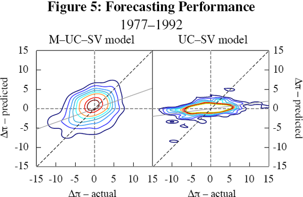
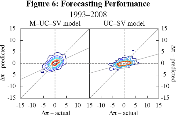
Figures 5 and 6 plot the actual change in inflation against the forecasted change. Because there are too many data points for a scatterplot to be meaningful, we show the contours of kernel density estimates instead. Following Theil (1966), the plots focus on the forecast of the change in inflation, rather than the forecast of its level, for several reasons: this puts the focus on predicting turning points, which is both harder and arguably more useful than predicting a continuing trend; it circumvents the problem of rescaling and demeaning the observations; and it makes it easy to visualise the naïve forecast (Δπ_t+8 = 0) that we use as a benchmark. To interpret these, note that a naïve forecast (which has π_t+8|t = π_t) would generate points along the horizontal axis, while a perfect forecast would be a 45° line through the origin. The solid line shows the line of best fit through each set of points. The gradient of this line of best fit is comparable to the forecastability measures of Theil (1966). It indicates how far the model's average performance is from that of a perfect forecasting model, with a value of one corresponding to perfection and a value of zero indicating failure.

These figures confirm that inflation became easier to forecast from the first half of the sample to the second; both lines of best fit for each model are closer to the 45° line. Overall, it seems that the M-UC-SV model's forecasts are less biased, at the cost of lower precision. This is evidenced by the fact that its line of best fit (solid line) is steeper than that of the UC-SV (M-UC-SV forecasts are more accurate on average), while the contours around these solid lines are wider (M-UC-SV forecasts are less precise). In other words, the UC-SV's forecasts of Δπ_t+8 are biased towards zero. The bias for both models is somewhat lower in the latter period of low and stable inflation.

Table 4 reports the slope of the line of best fit, calculated as for Figures 5 and 6. The results suggest that inflation became easier to forecast across the board.

Table 4: The Bias of Inflation Forecasts

		1977–1992	1993–2008
Inflation targeters	UC-SV M-UC-SV	0.16 0.37	0.29 0.46
Non-targeters	UC-SV M-UC-SV	0.07 0.34	0.29 0.50
Note: The bias is measured by the slope of the line of best fit for Δπt+8|t regressed on Δπt+8.

In order to investigate more carefully the relative performance of the UC-SV model and its M-UC-SV version, we provide a country-by-country breakdown of the forecast performance in Table 5, based on the RMSE. Table 5 also reports the forecast performance of a naïve forecast for inflation eight quarters in the future (π_t+8|t) based on the most recently observed value (π_t). In other words, it always predicts no change in inflation. We also present the RMSEs of a benchmark provided by the Atkeson and Ohanian (2001) (AO) model, whereby the eight-quarter-ahead inflation rate is forecast as the average rate of inflation over the previous four quarters.^[13]

Table 5: Root Mean Squared Errors

		1977–1992	1993–2008
Australia	AO	4.23	1.67
	Naïve	4.51	2.24
	UC-SV	3.77	1.81
	M-UC-SV	4.05	2.10
Austria	AO	2.57	1.70
	Naïve	3.09	2.08
	UC-SV	2.81	1.64
	M-UC-SV	2.34	1.56
Canada	AO	3.44	2.51
	Naïve	3.63	3.11
	UC-SV	3.46	2.45
	M-UC-SV	4.30	2.48
France	AO	3.37	1.37
	Naïve	3.43	1.76
	UC-SV	3.32	1.34
	M-UC-SV	4.53	1.54
Germany	AO	2.64	1.84
	Naïve	2.75	2.27
	UC-SV	2.65	1.82
	M-UC-SV	2.60	1.61
Japan	AO	3.63	1.80
	Naïve	3.86	2.16
	UC-SV	3.56	1.73
	M-UC-SV	3.17	1.56
NZ	AO	6.10	2.14
	Naïve	6.83	2.42
	UC-SV	6.62	2.14
	M-UC-SV	5.56	2.17
Sweden	AO	4.74	2.85
	Naïve	5.69	2.91
	UC-SV	4.59	2.86
	M-UC-SV	5.09	2.96
UK	AO	3.10	1.69
	Naïve	3.55	1.59
	UC-SV	3.35	1.44
	M-UC-SV	2.72	1.53
US	AO	2.06	1.60
	Naïve	4.21	1.85
	UC-SV	4.12	1.57
	M-UC-SV	3.78	1.47

We chose the AO model as a benchmark as it is hard to beat.^[14] Consider two extremes. If inflation were a random walk, the best forecast would be the current value of inflation (the naïve method), but the AO model would also do reasonably well. In contrast, if inflation was subject only to purely transitory shocks, the naïve method would do poorly, while again the AO model should do reasonably well. The M-UC-SV model should perform relatively well in situations where inflation experiences persistent (but not permanent) deviations from a relatively stable mean. Also, one advantage of the UC-SV and M-UC-SV models is that they can accommodate changes in the volatility of the persistent and transitory components.

Together, the two models outperform the AO benchmark in most countries in both sample periods. For Australia in the more recent sample period, the AO model performs best, and across all models the RMSE for Australia is comparable to those of Austria, Japan, the United Kingdom and the United States, and lower than for Canada, New Zealand and Sweden. Across all countries, the performance of the M-UC-SV is comparable to that of the UC-SV model. Excluding the countries where both models fail to beat the AO benchmark, the M-UC-SV is preferred to the UC-SV model in a majority of countries.

The ability of these models to outperform the AO benchmark in a range of countries is evidence against the conclusions of recent econometric studies (including Stock and Watson 2007). That literature suggests that inflation became easier to forecast in the sense that the size of RMSEs had fallen (as in Table 3 above) and that more stable inflation makes the AO model a harder benchmark to beat. By contrast, in our second sample period, the AO model is clearly superior in only one out of ten countries; the last few years of the sample show a rise in the persistent component of inflation for most countries, which the UC-SV and M-UC-SV models should capture better than the AO model.

Footnotes

The permanent component of inflation provides a h-period-ahead forecast measure of inflation (π_t+h|t = τ_t|t) for the UC-SV model. In the autoregressive version, the forecast is an exponentially weighted average of the persistent deviation τ_t and the permanent level μ. [12]

Here we follow Stock and Watson's (2007) interpretation of Atkeson and Ohanian (2001). [13]

Stock and Watson (2007, 2008) provide a comprehensive review of the forecasting performance of many inflation models (a total of 157 distinct models). They report that there is no single model, nor combination of univariate models, that has uniformly better performance than the UC-SV model, at least for quarterly US data. Canova (2007) focuses on CPI inflation in G7 countries and finds that the performance of univariate time-varying parameter models is hardly any different than that of more complicated model specifications. [14]