RDP 2006-06: Ageing, Retirement and Savings: A General Equilibrium Analysis 5. Results
July 2006
- Download the Paper 407KB
We now discuss the results from four scenarios, each of which deals with a different set of unanticipated demographic changes (Table 2). The first two scenarios involve changes in fertility. Of these, the first is a permanent fall in fertility. The second is a 20-year increase in fertility followed by a permanent fall to a value lower than the initial level – this is the baby ‘boom and bust’ characteristic of many developed countries after the second World War. The third scenario is an increase in longevity, which we model as an increase in T. It is more realistic to expect a rise in longevity to play out over the course of many years and be at least partially anticipated. However, even recently, official projections of longevity have been revised considerably over a short period of time.[17] The final scenario combines the second and third to examine the economic implications of an increase in longevity coupled with a baby boom and bust.
| Scenario | Values of demographic parameters | |||||
|---|---|---|---|---|---|---|
| Fertility parameter (per cent) | Longevity (years) | |||||
| n1 | n2 | n3 | T1 | T2 | ||
| 5.1 | 1.2 | 0.0 | 0.0 | 60 | 60 | |
| 5.2 | 1.2 | 2.4 | 0.0 | 60 | 60 | |
| 5.3 | 1.2 | 1.2 | 1.2 | 60 | 70 | |
| 5.4 | 1.2 | 2.4 | 0.0 | 60 | 70 | |
5.1 Permanent Fall in Fertility
In this scenario the fall in fertility is permanent, so the model shifts to a new steady state.[18] In steady state, aggregate variables grow at the rate of population growth, n, so a reduction in fertility decelerates the growth rate of these variables.
However, in the transition, different variables decelerate at different rates – and some even accelerate for a short while.
The fall in fertility acts like a reduction in labour supply. Workers become
relatively more scarce than they were initially, so the capital-to-labour ratio rises
relative to the initial steady state (Figure 3). Therefore, wages rise from their initial
level, and interest rates fall. These changes in factor prices induce shifts in the savings
and retirement behaviour of agents. For the latter, we find that the substitution effect
dominates the income effect from higher wages. As a result, agents retire slightly later in
the new steady state, with the share of life spent working (defined as  rising from 62.8 per cent to 63.0 per cent.
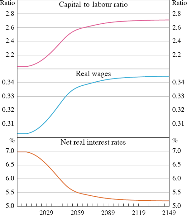
Figure 4 shows the lifetime profile of wealth, leisure and consumption in the two steady states. As we would expect, the consumption profile becomes flatter in response to lower interest rates. Higher wage rates induce agents to supply more labour and help them to accumulate more wealth over their lifetime. This in turn allows them to finance more consumption over their lifetime (notwithstanding the lower return to capital). In fact, agents in the final steady state are better off, in terms of lifetime utility, than agents in the initial steady state.
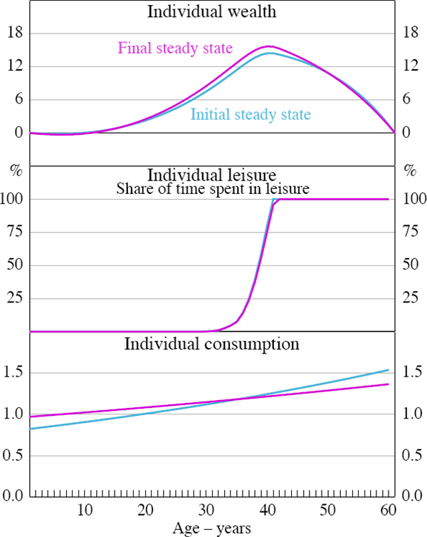
Note: The last period shown is 61 years when the person has died and has no wealth left.
To help understand the transition between the initial and final steady states, we can examine the growth rates of the capital stock and the labour supply (Figure 5). With the capital-to-labour ratio rising during the transition, we know that the growth rate of the capital stock must be above the growth rate of the efficient workforce during this period. In fact, the growth rate of capital rises above its initial level for about 15 years. That is, the growth rate of aggregate savings actually rises for a time. Different cohorts make very different contributions to this aggregate result. While younger cohorts increase consumption and reduce their saving rates during this period, this is more than offset by an opposing response of middle-aged and older cohorts.
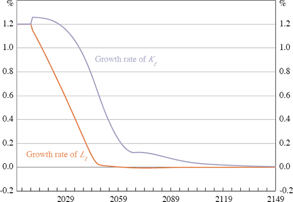
These responses from different cohorts occur because the changes in factor prices affect these two groups differently. Those in their middle and old age do not benefit as much as younger generations from the increase in wages, because much (or all) of their working life has already passed. Also, lower interest rates decrease current and future income, especially for those already retired, who depend entirely on income from capital. Middle-aged and older cohorts react by reducing consumption and increasing savings. Younger cohorts are harmed less by lower returns to capital since they have accumulated little or no wealth. For them, the increase in wages together with a high time endowment allows them to initially increase consumption and reduce saving.[19]
Although this model incorporates non-standard features, the result that a decline in population growth (with unchanged longevity) leads to a higher capital-to-labour ratio is similar to the result from a standard two-period Diamond OLG model.
5.2 Baby Boom and Bust
Here there is an increase in fertility that lasts for 20 years, followed by a permanent fall in fertility.[20] During the boom, agents act as if the higher fertility rate were to last forever. In other words, both of the changes in fertility are unanticipated.[21]
Our model behaves symmetrically in the sense that the effects of the initial boom are opposite to those discussed above. The boom acts as an increase in the labour supply. This change in the capital-to-labour ratio puts downward pressure on wages and upward pressure on interest rates. Following the argument above, but working in reverse, the growth rate of aggregate savings falls initially.
After 20 years of transition towards the new steady state implied by the higher fertility rate, there is an unexpected fall in fertility. Except for the position of the economy at the time of the change, the dynamics are exactly those of our first scenario. The following baby bust eventually reverses the effects of the temporary boom, leading ultimately to the same steady state as before.
Figure 6 illustrates the transition for all scenarios. Comparing the paths for capital intensity, wages, and the interest rate for this scenario with those for the previous one, we can see that the baby boom delays the onset of the new steady state caused by the permanent fall in fertility. Furthermore, the baby boom causes interest rates and wages to initially move in the opposite direction.
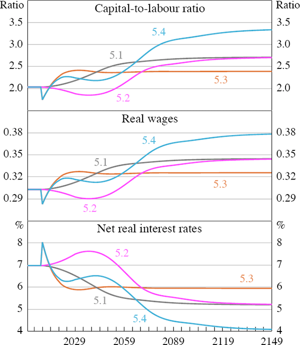
The economy eventually converges to the same final steady state as in Scenario 5.1, in which agents are better off than they were initially. However, the transitional dynamics in the two scenarios have quite different implications for the welfare of different cohorts.
5.3 Increase in Longevity
Here there is a permanent, unexpected increase in agents' lifespan, T. This is accompanied by an improvement in health, an assumption we relax later on. As agents are healthier and live longer, they retire later in life, increasing the aggregate labour supply. In response, wages jump down and interest rates jump up (Figure 6). However, these initial effects on factor prices are gradually unwound, so that eventually, wages rise and interest rates fall, relative to the initial steady state. This is because, in the longer run, increased longevity also raises the aggregate demand for labour. The mechanism at work is simple. A longer lifespan raises the absolute number of years agents spend in retirement. Agents must save more for this longer retirement, and these additional savings raise the aggregate capital stock. This in turn raises the marginal product of labour, which pushes up wages, and reduces the return on capital.
Interestingly, the share of life spent working is slightly lower in the new steady state. Agents are retired for 23 rather than 20 years, but work for 62.6 per cent rather than 62.8 per cent of their lives.
Figure 7 illustrates the differences in wealth accumulation, leisure, and consumption in the two steady states. Overall, agents accumulate more wealth, retire later, and have a flatter consumption profile.
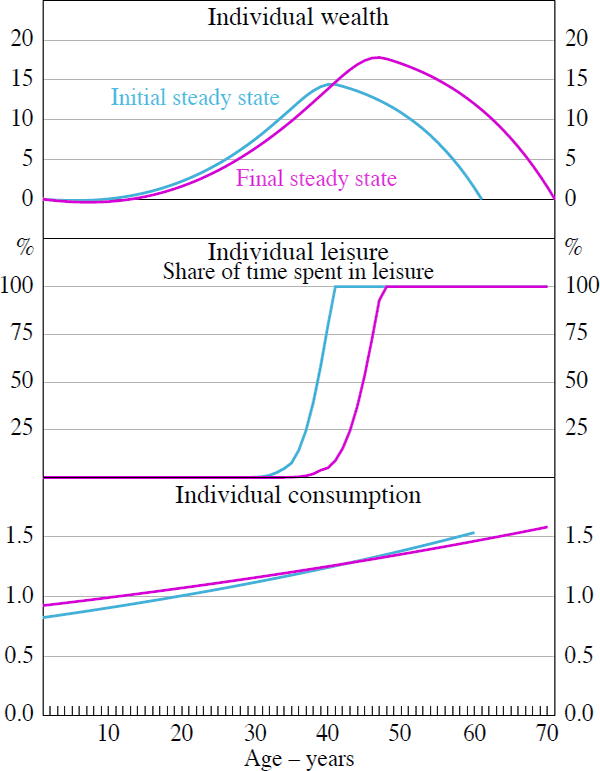
Note: The last period shown is 71 years when (under the higher longevity scenario) the person has died and has no wealth left.
We assume that all agents alive at the time of the change experience the same absolute increase in longevity. Both the fact that the change in longevity occurs suddenly rather than gradually, and the fact that it affects all agents equally, are not entirely realistic. Even so, the key results regarding the direction of changes in variables of interest should hold in a more realistic setting.
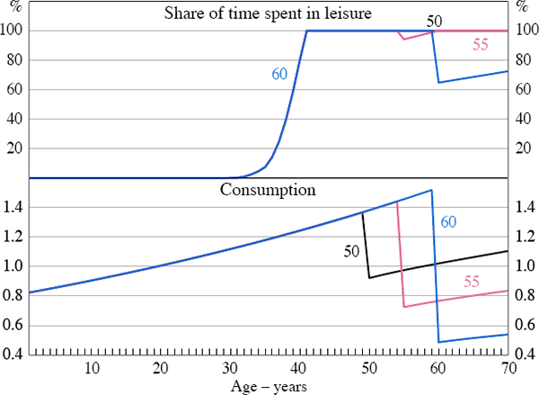
In our model, the labour supply response of older agents of different ages to the unexpected increase in longevity is particularly interesting. This is because there is a trade-off between reducing consumption and supplying labour which is wealth-and age-dependant. For example, those people who are 55 or above are already well into their retirement, having almost completely dissaved, and must return to work in order to finance consumption in these extra last years of their lives (Figure 8). As these people are at the end of their lives, their time-varying weight on leisure is very high. Agents aged about 50 at the time of the change also have a relatively high weight on leisure, but they have a larger stock of wealth than older retirees, so they choose to only cut consumption rather than return to work.
5.4 Combined Change in Fertility and Longevity
This scenario combines Scenarios 5.2 and 5.3 to investigate the economic effects of changes in fertility and an increase in longevity, which roughly characterises the demographic changes of the past half-century or so. We know that these two scenarios by themselves have the same sorts of effects: both an increase in longevity and a permanent baby bust will eventually raise wages, lower interest rates, and raise income and consumption per capita. More interesting is the fact that the effect of changes in fertility and longevity on variables such as the capital-to-labour ratio are not additive: the combined effect is greater than the sum of the two individual effects (Figure 6). In particular, the capital-to-labour ratio increases by 0.67 in Scenario 5.2, 0.35 in Scenario 5.3, and 1.32 in Scenario 5.4. However, the combined effect of a change in fertility and longevity on the steady-state retirement age is less than the sum of the two individual effects.
During the early part of the transition to the new steady state, there is a period of lower wages and higher interest rates driven by relatively abundant labour. In this scenario the increased labour supply has two sources: the temporary rise in fertility associated with the baby boom and the higher labour supply associated with increased longevity. Eventually, the lower fertility rates and the need to finance consumption over longer retirements raises the capital-to-labour ratio, increases wages and reduces rental rates on capital.
5.5 Sensitivity Analysis
Tables 3 and 4 illustrate the sensitivity of the steady-state capital-to-labour ratio and retirement behaviour to the demographic parameters in our model. We include some additional steady states not computed above. Comparing the capital intensities in Table 3 confirms that the results from the scenarios presented above hold more broadly. That is, both lower fertility rates and longer lives increase the capital intensity of the economy, and the effects of combined changes in longevity and fertility are superadditive. This result is, to the best of our knowledge, new in the literature.
| n (per cent) | T (years) | ||||
|---|---|---|---|---|---|
| 60 | 65 | 70 | 75 | 80 | |
| 2.4 | 1.55 | 1.65 | 1.75 | 1.85 | 1.94 |
| 1.2 | 2.04 | 2.21 | 2.39 | 2.60 | 2.77 |
| 0.0 | 2.71 | 3.03 | 3.36 | 3.73 | 4.12 |
| −1.2 | 3.67 | 4.21 | 4.81 | 5.48 | 6.20 |
| n (per cent) | T (years) | ||||
|---|---|---|---|---|---|
| 60 | 65 | 70 | 75 | 80 | |
| 2.4 | 62.5 | 62.3 | 62.2 | 62.0 | 62.0 |
| 1.2 | 62.8 | 62.7 | 62.6 | 62.6 | 62.5 |
| 0.0 | 63.0 | 63.0 | 63.0 | 62.9 | 62.9 |
| −1.2 | 63.2 | 63.2 | 63.2 | 63.2 | 63.2 |
| −2.4 | 63.3 | 63.3 | 63.3 | 63.3 | 63.4 |
Notice that in Table 3 changes in T do not leave the capital-to-labour ratio unchanged. One could choose quarters instead of years and recalibrate the rest of the parameters (by altering their units of account accordingly) so as to leave the capital-to-labour ratio unchanged. However, for a given choice of the unit of account for time, a change in T will not require a change in the the unit of account of the other parameters. For example, the rate of depreciation, and the magnitude of total factor productivity will be unchanged. For this reason, changes in T lead to a change in the capital-to-labour ratio.[22]
Table 4 shows the sensitivity of the time spent working to changes in the demographic parameters. For a given T, lower fertility decreases the share of life spent in retirement. This largely reflects the impact that higher wages associated with lower values of n have on labour supply decisions. Also notice that, for a given value of n, the share of life spent working can stay constant, rise, or fall with increases in longevity. This is because two opposing forces are at work. A longer lifespan provides more years over which to accumulate wealth from compounding interest income, but in general equilibrium a longer retirement increases the supply of capital and lowers the interest rates over which to compound. Interestingly, unlike Bloom et al's (2004) partial equilibrium analysis in which interest rates and wages remain constant, the share of life spent working in our model could move in either direction.
We also examine the sensitivity of our results to different parameter values and assumptions about health and human capital. Under the assumption that health does not improve when life expectancy rises, the capital-to-labour ratio converges to an even higher level than before.[23] An increase in lifespan of 10 years increases the steady-state capital-to-labour ratio from 2.04 to 2.39 when health improves and from 2.04 to 3.50 when there is no health improvement (Figure 9). With constant health, retirement behaviour is virtually unchanged relative to the initial steady state. That is, labour supply does not increase as much as in Scenario 5.3. Agents have an extra 10 years of consumption to finance but the amount of time spent in the workforce remains almost unchanged. As a result, they need to accumulate more wealth during their working lives.
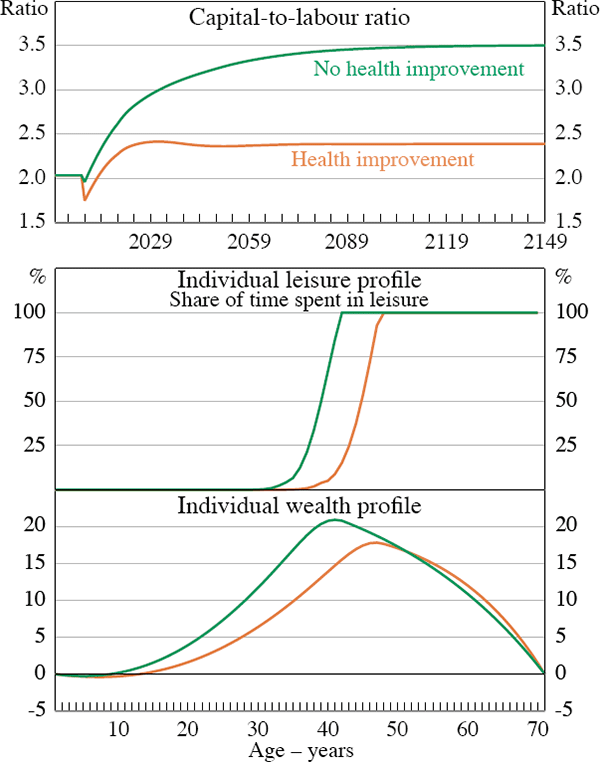
Note: The last period is 71 years when the person has died and has no wealth left.
With unchanged health, there is still an initial increase in the labour supply when longevity increases. The increased labour supply is mainly driven by older retirees' need to finance additional years of consumption despite their high disutility from working.
In steady state the profile of human capital operates (jointly with A) as a scaling parameter. However, in the face of (unexpected) lifespan changes, the profile of human capital is an important determinant of labour supply decisions. We investigate an increase in longevity and health under the assumption that, instead of rising over a person's lifetime, human capital remains constant (at the initial value of 2.5 in the benchmark calibration). We find that this lower level of human capital induces a stronger labour supply response to a change in T.
Our results are robust to a wide range of values for the other parameters.[24] For example, the qualitative results of Scenario 5.4 are robust to variation in the household's discount factor β; a rise in β from 0.97 to 0.99 increases the final steady-state capital-to-labour ratio from 3.33 to 5.09 and preserves the shape of the transition paths. The results are also robust to a lower value of ρ (1.5 compared to 3.5).[25]
Footnotes
For example, between 2001 and 2004, the Government Actuary's Department in the United Kingdom raised their projections for life expectancy for those reaching age 65 in 2050 by 4 years for women and 4½ years for men (Hills 2006). [17]
The model takes around 150 years to reach the new steady state in this scenario. Although population growth stabilises after around 70 years, the model takes longer than this to reach the new steady state. This is because, even after population growth has stabilised, there are agents still alive who have chosen their consumption and leisure sequences conditional on the non-steady-state price sequences of the transition period. [18]
Nevertheless, young people at the time of the change are worse off than subsequent generations. This is because factor prices adjust gradually. Hence those who are very young when the shock hits do not benefit from higher wages as much as future cohorts, and by the time they have accumulated a substantial quantity of savings, interest rates have fallen considerably. [19]
We choose a boom of 20 years to match the duration of the baby boom in Australia.
This simulation involves an additional complexity since it requires us to calculate a virtual future path of the economy which would not occur, but which is necessary to establish behaviour during the boom years. [21]
In Blanchard's (1985) model, where there is uncertainty about death, the effective discount rate becomes a function of the horizon (life expectancy) of agents. Although there is no uncertainty of this kind in our model, increasing β with T does not alter the result above – namely, that the capital-to-labour ratio rises with T. This result is a general one. It is easy to see why it holds in a very simple two-period OLG model, with non-productive, non-depreciating capital, a discount factor of one, a production function that is linear in labour, and assumptions about health such that people work for the first half of their lives. In this case, doubling the lifespan (to four periods) will double the (equilibrium) capital-to-labour ratio as agents now have to fund two consecutive periods in retirement. However, a four-period model could replicate the capital-to-labour ratio of the two-period model if agents were able to work in the first period, retire in the second, return to work in the third and retire again in the fourth. [22]
We model constant health by relaxing the assumption that ν(s, T) is homogenous of degree zero in s and T. We limit the dependence of v(.) on T by keeping the ‘mean’ and ‘standard deviation’ at their previous values (that is, b2T1 and b3T1 respectively). [23]
These additional results are available upon request. [24]
Much lower values of ρ were problematic for the convergence of the solution algorithm. In our model a lower ρ increases both the intra- and inter-temporal elasticities of substitution. Hence, the sensitivity of the inner and outer loops of the solution algorithm (illustrated in Appendix A) increase jointly when ρ falls. [25]