RDP 2006-06: Ageing, Retirement and Savings: A General Equilibrium Analysis 4. Calibration
July 2006
- Download the Paper 407KB
We choose values for the parameters so that the model's initial steady state would resemble key features of the current Australian economy. Parameter values (Table 1) were selected and constructed as follows:
| Variable(a) | Description | Value |
|---|---|---|
| T (years) | Life expectancy | 60 |
| n | Cohort growth rate | 0.012 |
| es | Human capital profile | See Figure 2 |
| b1 | Parameter of ν(s, T′) | 3.0 |
| b2 | Parameter of ν(s, T′) | 0.7 |
| b3 | Parameter of ν(s, T′) | 0.03 |
| β | Discount factor | 0.97 |
| ρ | Utility function parameter | 3.5 |
| A | Total factor productivity | 0.4 |
| 1 – α | Labour's share of income | 0.55 |
| δ | Depreciation rate | 0.052 |
| Note: (a) See Appendix B for detailed data sources and methods. | ||
Life expectancy (T)
The simple average of life expectancy at birth for males and females in 2003 is 80 years. As agents in our model begin life and work at the same time, and as it is reasonable to think that agents enter the workforce at around 20 years of age, we subtract 20 years from this lifespan to obtain an initial life expectancy of 60 in our model.
Cohort growth rate (n)
Our benchmark cohort growth rate (1.2 per cent per year) was calibrated so that the median age in the model is that of the 2004 Australian population, conditional on life expectancy. This strategy also yields a steady-state growth rate for the model population which is in line with the current growth rate of the Australian population.
Human capital profile (es)
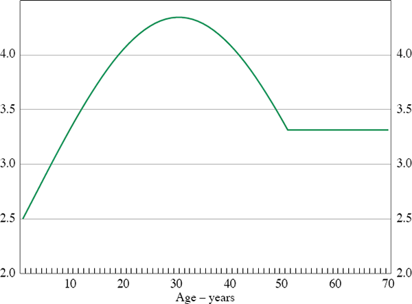
We approximate the level of human capital at each point in an agent's life using male and female age-wage equations estimated by the Australian Bureau of Statistics (ABS). These equations use cross-sectional data with the hourly wage as the dependent variable, and experience and education as independent variables. We assume no post-school qualifications (this alters only the level and not the growth of human capital over time) and construct hourly wages by age for a representative agent by weighting the estimated male and female wages by their share of hours worked.[14]
In the data used to estimate the ABS age-wage equations, the maximum work experience is 50 years, while agents can work for up to 60 in our benchmark steady state. Hence we needed to make an assumption about the out-of-sample path of human capital. We chose to hold human capital constant at its last observed value (Figure 2).

Note: In all figures, unless otherwise specified, the unit of measurement is in terms of the numeraire good (that is, output).
Time-varying weight on leisure: ν(s, T)
We choose b1, b2 and b3 in Equation (4) so that the leisure choices of an agent who lives their entire life under the conditions of the initial steady state broadly resemble the pattern of age-specific participation rates currently prevalent in Australia. At present, labour force participation begins to decline quite sharply when Australians are aged around 50 (30 in our model), and the average age of complete retirement is around 59 years (which means that some fraction of people aged 60 and above would still be in the workforce). We therefore choose b1,b2 and b3 (3.0, 0.7, 0.03) so that agents in the benchmark steady state begin to withdraw from the labour force at around 30 but are fully retired after 41 years, having worked for two-thirds of their lives.
Other utility function parameters: (β, ρ)
We choose a value of β (0.97) which is within the relatively narrow range of values used in the literature. In contrast, there is not much agreement with respect to the inter- and intra-temporal elasticities of substitution. For example, Auerbach and Kotlikoff (1987) discuss a range of studies where the inter-temporal elasticity varies from less than 1 to more than 14.[15] We choose a value for ρ (3.5) that generates a reasonable value for the capital-to-output ratio in the benchmark steady state. Our values of both β and ρ are comparable with those used by Auerbach and Kotlikoff. Our value of ρ implies an inter- and intra-temporal elasticity of substitution of 0.28. Auerbach and Kotlikoff set these values to 0.25 and 0.4 respectively.
Total factor productivity (A)
As discussed above, A is a scaling coefficient on output in OLG models of this kind. We chose a value of A (0.4) that generates broadly reasonable values for endogenous variables such as the capital-to-output ratio and the age of retirement in the benchmark steady state.
Labour share of income (1 – α)
Our value of 0.55 is the average of compensation of employees as a share of total factor income over 1995–2005.[16]
Real rate of capital depreciation (δ)
We choose 0.052, the average depreciation rate of the aggregate capital stock over 1995–2005. We average over this recent period because the depreciation rate has trended upwards since the early 1990s.
Footnotes
We experimented with adjusting females' work experience for child-rearing as discussed in Reilly, Milne and Zhao (2005). As the differences between the adjusted and unadjusted series are minor, we use the unadjusted values in our benchmark steady state. [14]
Most of these studies refer to models that do not have leisure in the utility function. [15]
This measure excludes labour's share of gross mixed income and net taxes on labour, which are properly included in labour's share of income. As these are positive in Australia, our measure probably slightly overstates the value of α. [16]