RDP 2005-04: Monetary Policy, Asset-Price Bubbles and the Zero Lower Bound Appendix C: Modelling Issues

In this appendix we briefly canvass three issues concerning our modelling framework and simulation results described in Sections 2 and 4.

The first is a technical caveat relating to the fact that the presence of the ZLB on nominal interest rates results in an activist policy-maker's expected loss ceasing to be a quadratic function of his contingent policy recommendations. This means that, in each period, not only must we resort to numerical methods to seek an activist's loss-minimising profile of contingent policy preferences, but we must also be concerned about the risk of inadvertently locating a local rather than global minimum. Moreover, this risk is likely to be even greater for the results in Sections 4.3 and (especially) 4.4 than for those in Sections 4.1 and 4.2, since the ability of policy-makers to influence a bubble's behaviour would already cause an activist's expected loss to cease to be a quadratic function of his contingent policy recommendations, even in the absence of the ZLB.

To help overcome this potential problem we adopted the following safeguards throughout the simulations reported in this paper. First, we set up the loss minimisation process using two different algorithms to provide a cross-check on our results.^[26] Secondly, having located notionally optimal sets of contingent policy preferences for each period, in a given scenario, we subjected these profiles to random perturbations to see whether re-optimisation starting from these perturbed settings would return the original profile, or instead give rise to an alternative with lower expected loss. Finally, these perturbation tests were separately carried out in various instances by each author so as to increase variety in the alterations tested. To the extent that these safeguards may have failed in any particular case, this would simply highlight the practical difficulties facing an activist policy-maker in trying to determine how best to respond to a developing asset-price bubble in the presence of the ZLB, even with perfect knowledge about both the structure of the economy and the stochastic properties of the bubble!

The second issue relates to the fact that, as discussed in Section 3.2.5 of Gruen et al (2003), there is a sense in which our baseline bubble considered in Section 4.1 could, under plausible assumptions about the relationship between the price growth underlying an asset bubble and the impact of that bubble on the real economy, be regarded as irrational. We do not see this as a shortcoming per se, since there is much evidence in developed economies of irrational bubbles occurring in practice – see, for example, Shiller (2000). Nevertheless, it is interesting to examine whether the imposition of a rationality assumption on our bubbles would affect the overall thrust of our findings.

As it turns out, simulations involving rational bubbles suggest that it would not – see Appendix C of Robinson and Stone (2005) for the details. It is important to note, however, that in asserting this we are not saying that, for activist policy-makers, their recommendations themselves (whether subject to a ZLB constraint or not) would be similar for a rational bubble and for our baseline bubble specified above. Indeed, the results in Section 3.2.5 of Gruen et al (2003) show that these recommendations would, in fact, be quite different. Rather, we are merely saying that, in terms of the marginal impact which the ZLB would have on the optimal recommendations of such activists, the nature of this impact is similar for both rational and irrational bubbles.

Finally, the third issue concerns the ‘threshold effect’ evident in Figure 7 in Section 4.4, and discussed briefly there. It is possible to understand more about both the precise timing of this effect, and its sensitivity to the model parameter λ, using the phase diagram introduced in Section 3 (Figure 1).

Regarding its timing, the issue is why an activist policy-maker, faced with the bubble in Section 4.4, should switch suddenly from recommending tighter policy than a sceptic in year 4, to sharply looser policy in year 5. It turns out that, in terms of Figure 1, this shift is driven by the activist's fear of allowing the economy to enter region II, where future policy would become constrained by the ZLB.

To see this, note that, if the bubble in Section 4.4 has not burst by year 4, then the sceptic's prior policy settings turn out to leave the economy at the point (0.30,0.85) in (y_t, π_t)-space by this time. This places the economy 4.33 percentage points horizontally to the right of region II in Figure 1 (for our economy with i* = 3, noting that line 2 in Figure 1 has slope −0.62). Hence an activist, in year 4, assesses that there is still scope to recommend slightly tighter policy than a sceptic, so as to increase the odds of the bubble bursting in year 5, without running any risk that the economy might be driven into region II were this to occur.

By contrast, if the bubble reaches year 5 without bursting, the sceptic's policy settings turn out to leave the economy at the point (0.20,0.97) in (y_t, π_t)-space, still only 4.43 percentage points horizontally to the right of region II in Figure 1. Since the negative shock to the economy were the bubble to burst next year is now 5 percentage points, this means that scope no longer exists for an activist to aim to burst the bubble by recommending tighter policy than a sceptic, without causing the economy to be driven into region II were he to succeed. It is this fundamental shift which governs the timing of the threshold effect evident in Figure 5, whereby an activist's optimal insurance strategy switches suddenly from trying to burst the bubble, up to and including year 4, to trying to create a buffer of higher inflation and output against its future collapse, from year 5 onwards.

A separate question is why an activist would be so fearful of entering region II when deciding how best to respond to the asset-price bubble of Section 4.4. This largely turns out to reflect the value of the parameter λ, which captures how ‘naturally self-correcting’ the real economy is, absent any policy action. For the simulation results shown in Figure 7 this parameter takes the value 0.8, which is quite close to 1. This means that an activist can expect the economy to recover only slowly of its own accord from a large negative shock. Hence the cost of entering region II, where policy would become constrained by the ZLB, would be substantial in this economy.

By contrast, in an economy with a lower λ this cost would be much less significant, so that concern about entering region II would weigh less heavily on the mind of an activist policy-maker. This point is nicely illustrated by Figure C1, which shows the analogue of Figure 7 for an economy with λ = 0.6, but with all other model and bubble parameters unchanged.

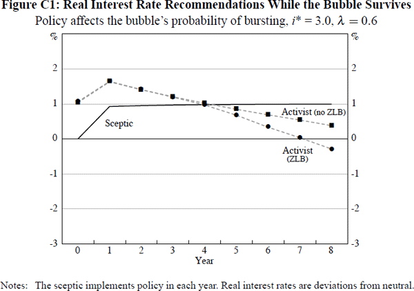
In this case the reduction in λ has several effects. First, as discussed in Footnote 18, it flattens lines 1 and 2 in Figure 1 (that is, makes their slopes less negative), so deferring slightly, to year 6, the time when an activist first perceives a risk of the economy being forced into region II by the bubble's collapse. More importantly, however, the reduction in λ substantially reduces the relative costliness of region II. Hence, rather than seeing a sharp threshold effect when this risk first arises, we see instead a measured, ongoing shift in an activist's optimal recommendations, away from trying to burst the bubble and towards building a buffer of higher inflation and output. Additionally, a further factor moderating the pace of this shift is that, as noted in Footnote 6, a lower value of λ reduces the cost-effectiveness of the buffer form of insurance against the ZLB when confronting an endogenous bubble.

Finally, on a quite separate point, it is interesting to note that a comparison of the results in Figures 7 and C1 does not alter our finding in Section 4.5 regarding the likely impact of changes in λ on the scale of the ZLB effect on an activist's recommendations. We see that, for the endogenous bubble considered in these figures, the absolute size of this ZLB effect is lower in every period for the activist in the economy with λ = 0.6 than for his counterpart in the λ = 0.8 economy. This is consistent with our results from the exogenous bubble case that the former activist will simply be less concerned about the ZLB than will the latter, who can expect less assistance in restoring output to potential, whenever the bubble bursts, from the economy's natural tendency to rebound from such a shock.

Footnote

Specifically, we set up the process using the ‘Solver’ function in Excel, which employs the Generalised Reduced Gradient (GRG2) optimisation algorithm, and using a manually coded steepest descent algorithm in EViews (into which we explicitly incorporated the ZLB constraint on policy-makers' permissible range of interest rate recommendations). [26]