RDP 2003-09: Housing Leverage in Australia 3. Preliminary Analysis

Before we outline an estimated model of household housing leverage in Section 4, we first present some stylised facts about Housing Leverage in Australia, identify some of the household characteristics likely to influence households' housing leverage, and undertake a brief graphical analysis of how three key variables – age of the household head, household income, and household housing wealth – are related to leverage.

According to the HILDA Survey the homeownership rate in 2001 was 68 per cent, broadly consistent with both the 2001 Census and the 1998 Household Expenditure Survey (HES). Of these owner-occupying households, 42 per cent were still paying off their home and a further 9 per cent had other kinds of debt secured against it, such as a second mortgage or home equity loan. Households with some leverage therefore represented around one-third of the households surveyed. The average level of household leverage implied by the HILDA data is a little below the level implied by the aggregate credit data, at around 15 per cent for all owner-occupying households. This is despite the inclusion of loans from friends and family that are not in the aggregate data; these account for just under half of a percentage point of the average. The leverage of only those households with outstanding debt on their owner-occupied home averages around 48 per cent, which given the definitional differences in the debt measure, is roughly consistent with aggregate figures.

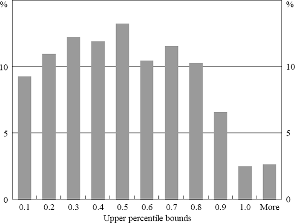
Although these figures confirm that, on average, housing debt is much lower than the value of housing assets, we are also interested in how this leverage is distributed across Australian households. Figure 1 shows that the distribution of leverage is fairly evenly spread, but few Australian households have high leverage, that is, an LTV ratio greater than 80 per cent.^[3] Only 11.4 per cent of households with housing loans (less than 4 per cent of all households) had an LTV ratio that exceeded 80 per cent, and less than 3 per cent had negative equity in their homes.^[4]

3.1 Leverage and Household Characteristics

We can use the wealth of cross-sectional information about Australian households contained in the HILDA dataset to investigate whether the diversity of household leverage is related to observable characteristics.

There are a number of household characteristics that can be expected to influence housing leverage. First, we would expect leverage to be affected by a household's stage in the life cycle. Leverage should be low for young households because their homeownership rates are low; few younger households would have saved enough to purchase a home while they are still completing their education and establishing their careers. Indeed, younger people may not have formed households at all for these reasons. Leverage should then rise as households move into their peak family formation years. This usually occurs early in their working lives when they have accumulated little wealth, so they must borrow to purchase large assets such as the family home. This debt is then steadily reduced over their working lives so that they are relatively debt-free when their incomes drop sharply upon retirement.

Variables that capture a household's position in the life cycle, such as the household head's age, labour force status, and marital status should therefore be important in explaining housing leverage. We also expect that the time since the mortgage was taken out, which we proxy using time the household has lived in the home, will be an important determinant of household leverage.

A household's means, and in particular its income, should also affect its leverage by influencing its willingness, need and ability to take on housing debt. We expect leverage to increase with income for three main reasons. First, higher-income households are more likely to be homeowners in the first place, because they are more likely to have been able to save the necessary downpayment. Second, we expect households that have paid off their mortgages to have lower incomes than households with existing mortgages, because retired lower-income households prefer to have paid off their debt. Finally, housing leverage may be expected to increase with income if financial institutions apply easier lending criteria to high-income households. The expected importance of household means in predicting leverage also leads us to anticipate that alternative indicators of household means, such as self-assessed income adequacy and the past occurrence of family breakdown should also influence leverage. Offsetting this, high-income households have more scope to pay off their loan quickly and thus own their home outright.

Finally, we would expect households' attitude to homeownership and debt to influence their housing leverage. For example, households that are uncomfortable about taking on debt may accumulate more savings before purchasing a home than households that feel more comfortable taking on debt. They may also choose to pay their loans off faster. Other variables that may pick up different attitudes to homeownership or debt across households include households' ethnic background, aversion to risk, and credit card usage.

3.2 Graphical Analysis

In Section 3.1 we identified a number of household characteristics that can be expected to influence a household's housing leverage. Before using this information in an econometric model, it is worth examining graphically how three key variables – age of the household head, household income, and household housing wealth – are related to housing leverage, treating households without mortgages as having zero leverage.

3.2.1 Age of the household head

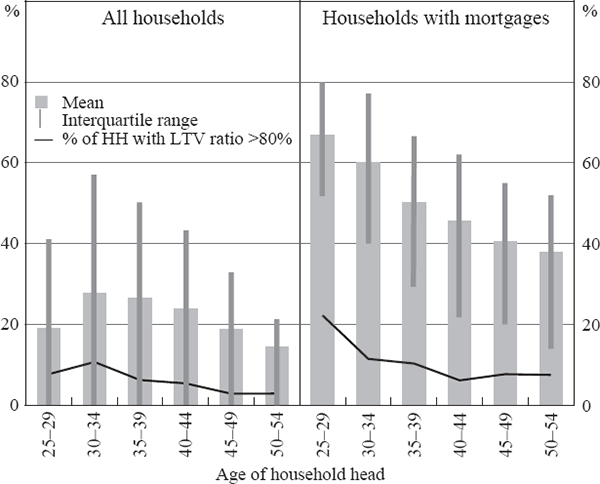
Figure 2 shows how housing leverage varies across age cohorts. In addition to mean leverage for each cohort we also include information about the distribution of leverage – the interquartile range, and the percentage of households with an LTV ratio greater than 80 per cent. The right-hand panel contains data only for households with mortgages, while the left-hand panel includes all households.

Looking first to the right panel, younger households with mortgages appear to have higher leverage than their older counterparts. Average leverage was almost 70 per cent for households where the household head was aged between 25 and 29, compared with 40 per cent for households with a head aged between 45 and 49. Similarly, younger households are more likely to have high leverage. Just under one-quarter of leveraged owner-occupying households with heads aged between 25 and 29 had leverage exceeding 80 per cent, a number that falls to just under 8 per cent for households with heads aged between 45 and 49. Because there is some association between age of the household head and time spent in homeownership, it is difficult to distinguish whether this is a pure age effect, or a reflection of the time the household has had to pay off their initial loan. This issue will be investigated in our econometric analysis in the following sections.

The left panel of Figure 2 shows that when younger households' lower homeownership rate is taken into account, their apparent higher leverage is reduced, and the nature of the relationship between age and leverage changes. Average leverage now increases to a peak when the household head is aged 30 to 34 before falling away as households pay off their housing debt. This observation is important because it shows that if we use a sample that only includes households with mortgages, we may exaggerate the incidence of leverage for categories of households with low homeownership rates, or higher rates of outright ownership where the mortgage has already been paid off. In our graphical analysis we make use of both samples so that we can observe pockets of high leverage in categories that otherwise have low debt. Similarly, in our empirical analysis, we use a technique that enables us to capture both the marginal effect of variables on leverage for those who have debt and the effect of these variables on the probability of having debt, giving us the total effect of variables on leverage.

3.2.2 Household income

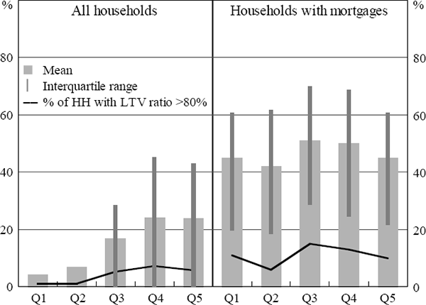
Figure 3 suggests that there may be a hump-shaped relationship between household income and leverage. Average leverage is greatest among upper-middle income households, and falls away somewhat for both low-income and high-income households. When the lower homeownership rate and share of households with existing loans in the bottom two income quintiles is taken into account (left panel), their average leverage looks particularly low. This may be partly an age effect; the average age of household heads in quintiles 1 and 2 is higher (at 55) than in the three higher income quintiles (at about 42).

3.2.3 Housing wealth

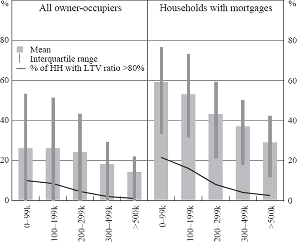
Although the Wave 1 HILDA Survey did not ask households about their non-housing wealth, their estimates of the current market value of their homes should capture a large proportion of their assets. According to Figure 4 there is a strong negative relationship between households' housing leverage and the value of their properties. Households with properties worth less than $100,000 had an average leverage (at almost 60 per cent) roughly double that of households with properties worth in excess of $500,000. The low average incidence of leverage among households with expensive properties is reflected in the much lower likelihood of their being leveraged above 80 per cent, at 3 per cent compared to over 20 per cent for households with homes worth less then $100,000. However, because owner-occupying households that have paid off their mortgages were more likely to have homes worth less than $100,000, their average leverage falls to about the same amount as households with homes worth between $100,000 and $199,000 when this is taken into account (left panel).

There are a couple of possible explanations for the negative relationship between housing wealth and housing leverage. First, if a household's housing wealth is positively correlated with its age and tenure length, then the observed relationship may only suggest that younger households, which are more likely to be highly leveraged, are also more likely to own cheaper homes. Second, if more expensive homes have appreciated more rapidly than less expensive homes, households that own more expensive homes will have experienced a larger passive reduction in their leverage, for a given length of tenure. Shocks to the price of a particular home have the opposite effect on the leverage ratio. If households update their assessments of their homes' current value for past price changes without adjusting their housing debt, this could generate a negative relationship between current estimated housing wealth and leverage.

One possible implication of the negative relationship between leverage and housing wealth is that leverage might be lower in locations with the highest housing prices, holding everything else constant. It is these areas – New South Wales and Victoria, and the inner suburbs of state capitals – that have experienced the strongest rises in housing prices recently, and thus where passive reductions in leverage are likely to have been greatest. In general, the data support this argument. Average leverage is relatively low in New South Wales and Victoria, and particularly in their inner-city suburbs, as is the incidence of high leverage. For example, in the late 2001 fieldwork period of this survey, average leverage for households with leverage in inner Melbourne was around 35 per cent (38 per cent in inner Sydney), compared to over 50 per cent in inner Brisbane and Adelaide. Indeed, only 1 per cent of households living in inner Melbourne in late 2001 had an LTV ratio above 80 per cent.^[5] Provided the average length of tenure (i.e., the frequency of households' decisions to trade up) is not greatly affected by the rate of house price inflation, this provides some comfort that those areas where concerns about future reversals of past price increases might be greatest are those where the negative equity consequences are least. This strengthens our general conclusion that the moderate level of aggregate Housing Leverage in Australia does not seem to be masking important pockets of potential vulnerability.

Footnotes

Our use of an 80 per cent threshold is consistent with evidence in Genesove and Mayer (1997) that household behaviour alters when leverage exceeds this level, and it allows us to consider how the incidence of negative equity might change if house prices were to fall by a significant amount. It is also the threshold above which borrowers require mortgage insurance. [3]

There may be other households with high leverage against other properties not captured here, such as an investment property. Unfortunately this possibility cannot be explored until Wave 2 HILDA data, including information on wealth, are released in late 2003. [4]

Classifying postcodes into inner and outer city groups requires some subjective judgment. We defined suburbs as inner city if they were fairly close to the CBD and considered prestige or fashionable places to live; the specific allocation of postcodes is available from the authors. [5]