RDP 9409: Default Risk and Derivatives: An Empirical Analysis of Bilateral Netting 4. The Effects of Netting on Credit Exposure
December 1994
- Download the Paper 105KB
This section aims to provide some intuitive understanding of the impact on the credit risk of a swaps portfolio in moving from a non-netting to a netting environment.
It is clear that current credit exposure is reduced by netting, so long as the portfolio is not comprised of contracts that are all on one side of the market; the magnitude of the reduction in credit exposure depending upon the value of the out-of-the-money contracts.
Consider the following portfolio of four swaps:
| Swap | Counterparty | Market value ($) |
|---|---|---|
| 1 | A | +10 |
| 2 | A | −10 |
| 3 | B | +10 |
| 4 | B | −10 |
In the absence of netting, the current credit exposure of the portfolio is equal to $20 (the sum of swaps with a positive replacement cost, there is no credit risk in swaps with a negative value). If netting is applied, then the credit exposure of the portfolio is reduced to zero (the positive and negative exposures to each counterparty offset each other).
The effect of netting on potential exposure is less clear, as it depends on the composition of the portfolio. There are two simple ways to look at the behaviour of potential exposure: firstly, through the use of projections of the value of a portfolio over some worst case interest rate scenario, as discussed in Section 3.3 above; and secondly by looking at the statistical behaviour of changes in the value of a portfolio.
4.1 Worst Case Scenarios
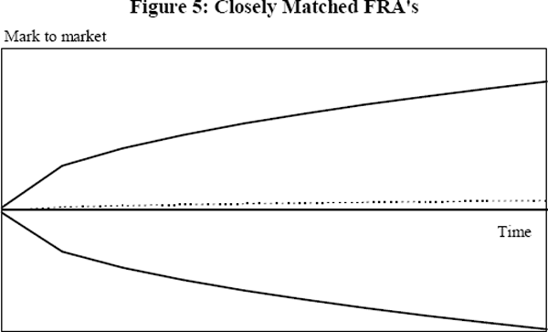
The following two figures present the worst case time paths of credit exposure for two FRAs (the solid lines) and the worst case time path for the net exposure on the two contracts (the broken line). Maximum potential credit exposure is equal to the maximum exposure obtained over the life of the contracts.
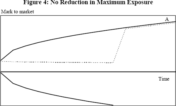
It is possible to envisage situations where a portfolio is comprised of contracts on opposite sides of the market, but maximum exposure is not reduced because that occurs after the maturity of the contracts that are out-of-the-money. Figure 4 illustrates this. In the absence of netting, total credit exposure is equal to the exposure on the positively valued contract (the upper solid line). Once the two contracts are netted, credit exposure (the broken line) on the portfolio is reduced over the life of the negatively valued contract. But, the portfolio exposure reaches the same maximum (point A) irrespective of whether or not the portfolio is netted. Average exposure, however, is reduced.
If deals between a bank and its counterparty are perfectly offsetting, netting eliminates current and potential exposure. Figure 5 shows the credit exposure on closely matched FRAs with the same maturity date. In this case, both the maximum and average potential exposure are greatly reduced when the contracts are netted. The more strongly correlated the two contracts, the greater the reduction in credit exposure. Table 3 contains the correlation coefficients between monthly changes in Australian interest rate swap rates and government bonds of varying maturities between February 1990 and September 1993. It can be seen that, over this period at least, swap rates across different maturities are, in fact, quite highly correlated.
| Swaps | Bonds | |||||||||||
|---|---|---|---|---|---|---|---|---|---|---|---|---|
| 6M | 1Y | 2Y | 3Y | 4Y | 5Y | 7Y | 10Y | 1Y | 5Y | 10Y | ||
| Swaps | 6M | 1 | ||||||||||
| 1Y | 0.874 | 1 | ||||||||||
| 2Y | 0.821 | 0.981 | 1 | |||||||||
| 3Y | 0.811 | 0.968 | 0.995 | 1 | ||||||||
| 4Y | 0.817 | 0.956 | 0.985 | 0.994 | 1 | |||||||
| 5Y | 0.808 | 0.945 | 0.975 | 0.986 | 0.996 | 1 | ||||||
| 7Y | 0.756 | 0.895 | 0.931 | 0.942 | 0.964 | 0.970 | 1 | |||||
| 10Y | 0.682 | 0.812 | 0.856 | 0.871 | 0.905 | 0.920 | 0.976 | 1 | ||||
| Bonds | 1Y | 0.949 | 0.957 | 0.922 | 0.909 | 0.903 | 0.892 | 0.849 | 0.775 | 1 | ||
| 5Y | 0.806 | 0.943 | 0.971 | 0.979 | 0.988 | 0.986 | 0.967 | 0.925 | 0.902 | 1 | ||
| 10Y | 0.618 | 0.750 | 0.794 | 0.806 | 0.839 | 0.853 | 0.931 | 0.967 | 0.726 | 0.877 | 1 | |
4.2 Changes in the Value of a Portfolio
The second way of looking at potential exposure follows from the observation that potential exposure can be closely linked to the market risk facing the portfolio. Consider a bank that has contracted, as the result of an interest rate swap, to receive fixed rate payments in exchange for floating rate cash flows. If the swap rate falls the bank profits – it could enter into an offsetting swap at the lower rate and lock in a profit equal to the difference between the initial swap rate and the current market rate. The bank has gained from the movement in market rates. However, if the counterparty defaults the bank loses those profits. This is credit risk. When the swap rate rises the bank incurs a loss – if it were to enter into an offsetting swap it could only do so at a loss. This is market risk. This paper is concerned only with credit risk. However, the analytical tools developed for evaluating market risk are useful in investigating the behaviour of potential credit exposure.
Hence, another way of looking at potential exposure is to consider changes in net replacement cost.[8] The more volatile the change in net replacement cost the greater the potential credit risk. While netting may, therefore, reduce the level of the current credit risk of a swap portfolio, that fact says little about potential exposure since it is determined by changes in net replacement cost. This volatility is determined by the volatility of the contract rates and the correlation between those rates.
Under a netting agreement the changes in the values of swaps, both in and out-of-the-money, are summed. In the absence of netting, current net replacement cost is calculated by summing all positive swap values and ignoring all negative swap values (that is, those that are out-of-the-money). Without netting, the change in net replacement cost is approximately the sum of changes in the values of in-the-money swaps. There is no reason to believe that the volatility of positive valued swaps is any larger, on average, than the volatility of all swaps (which determines potential exposure in the presence of netting). This suggests that the adoption of netting will not necessarily lower potential exposure.
Consider again the portfolio of swaps presented above in Table 2. Suppose that each of the swaps has the same variance so that its value can be expected to move up or down in value by $4 in the next year. Assuming that the movements in the value of each swap are independent, then there are sixteen possible outcomes at the end of the year. These are shown in Table 4. In the absence of a netting agreement, there are four cases when the credit exposure of the portfolio rises by $8 and four when it falls. With netting there are four cases where credit exposure rises by $8 and one case where credit exposure rises by $16. In no single case does it fall.
| Counterparty A | Counterparty B | Without netting | With netting | |||||
|---|---|---|---|---|---|---|---|---|
| Swap 1 |
Swap 2 |
Swap 3 |
Swap 4 |
Portfolio credit exposure |
Change |
Portfolio credit exposure |
Change |
|
| Initial swap value |
10 | −10 | 10 | −10 | 20 | – | 0 | – |
| Case | Possible swap values | |||||||
| 1 | 6 | −14 | 6 | −14 | 12 | −8 | 0 | 0 |
| 2 | 14 | −14 | 6 | −14 | 20 | 0 | 0 | 0 |
| 3 | 6 | −6 | 6 | −14 | 12 | −8 | 0 | 0 |
| 4 | 14 | −6 | 6 | −14 | 20 | 0 | 0 | 0 |
| 5 | 6 | −14 | 14 | −14 | 20 | 0 | 0 | 0 |
| 6 | 14 | −14 | 14 | −14 | 28 | 8 | 0 | 0 |
| 7 | 6 | −6 | 14 | −14 | 20 | 0 | 0 | 0 |
| 8 | 14 | −6 | 14 | −14 | 28 | 8 | 8 | 8 |
| 9 | 6 | −14 | 6 | −6 | 12 | −8 | 0 | 0 |
| 10 | 14 | −14 | 6 | −6 | 20 | 0 | 0 | 0 |
| 11 | 6 | −6 | 6 | −6 | 12 | −8 | 0 | 0 |
| 12 | 14 | −6 | 6 | −6 | 20 | 0 | 8 | 8 |
| 13 | 6 | −14 | 14 | −6 | 20 | 0 | 0 | 0 |
| 14 | 14 | −14 | 14 | −6 | 28 | 8 | 8 | 8 |
| 15 | 6 | −6 | 14 | −6 | 20 | 0 | 8 | 8 |
| 16 | 14 | −6 | 14 | −6 | 28 | 8 | 16 | 16 |
Using this simple example, we see that the change in credit risk on a netted portfolio is at least as large as the non-netted case in all but one of the sixteen cases. This is in spite of the fact that the level of exposure with netting is less than the level without netting in every instance.
More generally, Estrella and Hendricks (1993) demonstrate that, in the case where the swaps making up a portfolio are uncorrelated, then the variance of the portfolio's value does not change when moving from a non-netting to a netting environment.
An important caveat is that, rather than being independent, changes in swap values tend to be positively correlated. The greater the correlation between swap prices the greater the reduction in the variability (and hence potential exposure) of the swaps portfolio under netting. As shown in Table 3 above, swap rates do tend to be quite highly correlated.
Footnote
This section draws heavily from Hendricks (1992). [8]