RDP 9409: Default Risk and Derivatives: An Empirical Analysis of Bilateral Netting Appendix 1
December 1994
- Download the Paper 105KB
A1.1 Interest Rate Model
The model used to generate the time paths for interest rates is that used by the Federal Reserve Bank of New York (FRBNY) in some of its work on netting. This model incorporates a simple curved and varying term structure.[20] The two end points of the yield curve are allowed to vary stochastically over time and all points between these two are determined by an exponentially weighted average of those two yields.
Movements in the short yield are assumed to be driven by two factors. Firstly, the short yield is taken to drift towards the current long yield at a fixed speed determined by the parameter k. Secondly, a random shock, ε , is added to this process. The standard deviation of this shock is taken to be proportional to the short yield. The discrete approximation to this process is:

where:
| t | denotes time; |
| St | is a short yield; |
| Lt | is a long yield; |
| ε | is a standard normal deviate; and |
| k | is the rate of reversion of the short rate towards the long rate. |
The long yield is modelled as geometric Brownian motion with no drift.

where:
| dz | is a Wiener process. |
Hence the logarithm of the long rate can be taken to be distributed normally:

where:
| Mt | = ln(Lt); and |
| M0 | is the current value of M. |
While the long rate is characterised as geometric Brownian motion with no drift, there is drift in the process determining the log of the long rate, Mt. This drift term, −σ2t, is reflected in the simulation process to prevent the simulated interest rate paths from drifting upwards. The stochastic processes ε and dz are assumed to be independent.
Given a short and long yield, yields for any maturity are derived using the following equation:

where:
| y(τ) | denotes the yield for maturity to τ.[21] |
Parameters for this model were obtained using weekly observations of the 90-day bank bill rate and the ten-year government bond rate over the period January 1984 to August 1993. σ was estimated to be equal to 0.1, and k was estimated at 0.46. Initial values for the short and long rates were set at 4.75 per cent and 6.82 per cent respectively.[22]
The confidence interval on the short rate is derived from simulations of equation (A1). The confidence interval on the long rate can be obtained directly from equation (A3). For the purposes of the analysis, two worst case interest rate scenarios are considered: firstly, both short and long rates track the upper band of their 95 per cent confidence intervals; and secondly, both short and long rates fall to the lower extreme of their confidence intervals. For each contract we calculate replacement cost at weekly intervals over the life of the contracts for the two interest rate scenarios.
A1.2 Setting the Swap Rate
The interest rate model above determines the yield curve for zero coupon interest rates. To revalue an interest rate swap it is necessary to derive a swap rate from the zero coupon rates.
A fixed-to-floating swap can be characterised as a combination of a standard fixed interest bond and a floating rate note. The fixed rate side can be valued using traditional security valuation techniques based on present value concepts. Valuation of the floating rate side is complicated by the fact that the expected cash flows are not certain as they are contingent on the level of future interest rates. We assume that the floating rate component has been reset to par (notional face value) since the floating rate side is frequently repriced.
Hence, the current market price of the swap, P0 can be written as:
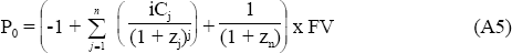
where:
| zj | denotes the zero coupon rate applicable to a cash flow occurring at time j; |
| n | denotes the total number of coupons payable under the swap; |
| Cj | is equal to the jth coupon period; |
| FV | is the notional principal amount; and |
| i | is the swap rate.[23] |
To determine the swap rate, i, we assume that at the date the swap is written the swap rate is set such that the current market price of the swap is zero. That is, equation (A5) is solved for i setting P0 equal to zero. In theory competitive forces within the swap market should ensure that this condition holds.
For example, consider a 3-year swap, written on 20 September 1992 with fixed rate payments payable semi-annually, and the following zero coupon rates substituting these values into equation (A5) and setting P0 equal to zero yields a swap rate of 5.57 per cent.
| Coupon dates |
Zero coupon yield curve Zj |
Coupon period (years) Cj |
|---|---|---|
| 20 Mar 92 | 4.96 | 0.4986 |
| 20 Sep 92 | 5.15 | 0.5041 |
| 20 Mar 93 | 5.30 | 0.4959 |
| 20 Sep 93 | 5.44 | 0.5041 |
| 20 Mar 94 | 5.56 | 0.4959 |
| 20 Sep 94 | 5.67 | 0.5041 |
To summarise the process for an individual contract: at each point in time, a worst case zero coupon yield curve is observed. From that yield curve, a swap revaluation rate is calculated which is the market rate to replace the remaining cash flows of the swap. The present value of the difference between the swap's cash flows and the payments made under the replacement swap is calculated to give the value at risk if the counterparty were to default. These steps are repeated at weekly intervals over the life of the swap to generate a time path for the credit exposure of the contract.
Footnotes
The FRBNY has conducted work using this model and the more sophisticated model developed by Longstaff and Schwartz (1992). While the simpler model we use lacks the theoretical rigour of the latter model the FRBNY found that, for their work, the two models yielded similar results. [20]
Note that the model's long rate is in fact the rate on a security with infinite
term to maturity, that is, y(t) = Lt only when t → ∞. Equation (3) can be modified so
that y(10) = Lt by replacing Lt with  where
where  and f = (1 –
e−10k)/10k. That is equation (3) is rewritten as
y(τ) = L* + (S – L*)
and f = (1 –
e−10k)/10k. That is equation (3) is rewritten as
y(τ) = L* + (S – L*) . For our simulations we do not
employ this adjustment, but simply use equation (3) above.
[21]
. For our simulations we do not
employ this adjustment, but simply use equation (3) above.
[21]
These values compare with estimates obtained using US data for σ and k of 0.1 and 0.3 respectively. [22]
This is an extension of the formula given in Das (1994) p. 192. [23]