RDP 8601: New Classical Models and Unobserved Aggregates 4. Persistence of Expectational Errors and Demand Shocks

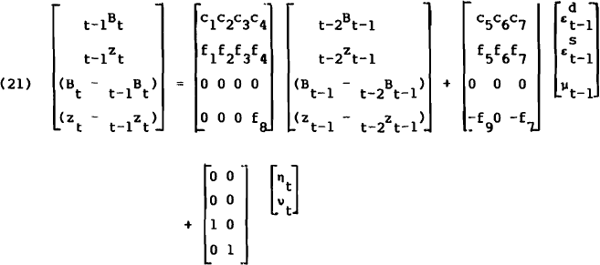
The solutions to the equations at the end of Section 2 required expressions for _t−1B_t and _t−1z_t. These can now be obtained by applying the expectations operator to equations (6) and (7) and using equation (19) to substitute out for _t−1z_t−1. The model may then be represented by the block-recursive, vector-autoregressive process

and

where the elements of the coefficient matrices are given in the Appendix.

The conditions required for covariance stationarity of this system of equations are that the roots of the quadratic

lie within the unit circle,^[12] with the additional restriction that

that is,

It was the assumption of these three conditions that allowed a stationary solution to the Kalman filtering problem to be calculated. These stationarity assumptions are maintained for the remainder of the analysis.

The solutions for the left-hand side variables of (21), and hence (20), will generally be infinite moving averages of terms in and [η_t, ν_t ]'. The first result of the model follows from this property. The unanticipated multiplier is not a white noise disturbance, as it would be in a standard New Classical model, but the infinite moving average process

where Σ_i is the sum from zero to infinity. Therefore, the error in the rational expectation of the true money stock is

Both of these expectational errors exhibit serial correlation. Yet it is traditionally thought that the assumption of rational expectations, and hence the application of the “orthogonality principle”,^[13] ensures white noise expectational errors. However, this assumption only rules out serially correlated expectational errors when the lagged values of these errors are included in the information set. In this model M_t−1, and z_t−1, are not in the agents' information set; hence nor are the lagged values of these expectational errors. In such a situation this analysis shows that the assumption of rational expectations does not necessarily prevent the occurrence of serially correlated expectational errors.

Combining equations (20) and (22) gives the second result,

That is, output contains an infinite moving average of demand disturbances, with geometrically declining weights. This persistence of demand shocks is due entirely to the unobservable nature of the true monetary aggregate. Agents only see partial information, from which they must filter out the “signal” from the “noise”, to generate optimal guesses about the unobserved variables. The persistence does not depend on the parameterisation of the measurement error in equation (8) – that is part of the information that can be filtered out. It does depend on the appearance of some lagged value of the true multiplier in its own reduced form, equation (7).^[14]

This result is for the stationary solution of the Kalman filtering problem. Outside of this stationary state, the weights in the moving average will vary each period as the filtering error variances change (equations (15), (16) and (17)). In such a situation, output will respond to demand shocks with long and variable lags. This confirms a conjecture of Lucas (1977):^[15]

These remarks do not, of course, explain why monetary effects work with long and variable lags. On this question little is known. It seems likely that the answer lies in the observation that a monetary expansion can occur in a variety of ways, depending on the way the money is “injected” into the system, with different price response implications depending on which way is selected. This would suggest that one should describe the monetary “state” of the economy as being determined by some unobservable monetary aggregate, loosely related to observed aggregates over short periods but closely related secularly.

Footnotes

In the special case where the authorities adjust the monetary base only in response to lagged values of itself and output (π=ρ=τ=0), these two conditions collapse to requiring that |θ| and |φ+ψ| both be less than unity. [12]

This is the term given by Sargent (1979, p.204) to the fact that the projection (rational expectation) error is orthogonal to every element of the information set, and therefore to the projection itself. Intuitively, if this were not true, the projection would not have utilised all the relevant information assumed available to the agents and in this sense would not be “rational”. [13]

This persistence result depends on some direct intertemporal linkage of the unobserved variables. In this model, such a linkage exists when φ is non-zero. In an expanded model where the aggregate price index is also measured imperfectly, the linkage could be provided by the parameter ψ in equation (7). [14]

Emphasis in original. [15]