RDP 8601: New Classical Models and Unobserved Aggregates Appendix

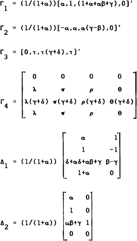
The coefficient matrices of the compacted model given in equation (12) are

To solve for the recursive set of equations that determine the vector of Kalman filter weights, use equations (11) and (12) to give

and

Using these two equations to evaluate the variance and covariance terms needed in (14) yields

and

Denoting var , and substituting these expressions into (14) gives

as the expression for Kalman coefficients. Taking the variance of both sides of equation (A1) results in

or, more compactly

Using the filtering formula (13) to substitute out for _tz_t shows that

Taking variances of both sides and noting the definition in (14) gives

or in compact notation

In order to derive the covariance stationary solution to the recursive Kalman filter given by equations (13), (15), (16) and (17), combine equations (15) and (17) to get,

and then use (16) to yield,

The stationary solution for is then the solution to the quadratic in σ²,

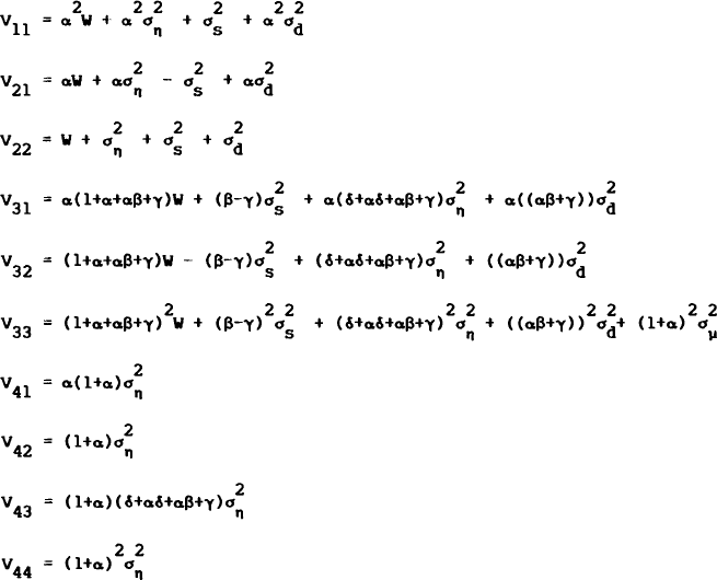
Denote the matrix by V. This is the symmetric matrix var(x_t − _t−1x_t) and by using the definitions in equation (12) its lower triangular elements are Found to be (1+α)⁻² times the following entries,

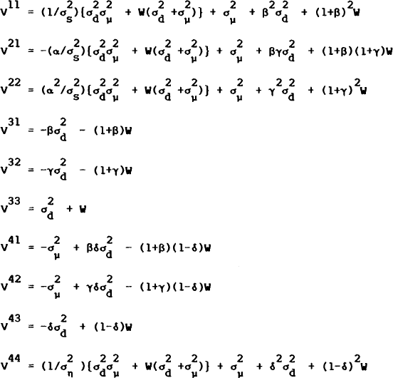
where . The inverseof V may be found by a sequence of elementary row operations.
Its elements are  times the entries,

Substituting back into equation (A4) gives,

which is the quadratic in σ²,

The stationary solution for σ² is then the positive root of the solution^[28]

Given this stationary solution for σ², the stationary solution for the Kalman weights may be found by substituting into equation (15)

Judicious use of equations (A5) and (A6) reduces this to

which proves the Lemma in the text. Substituting these weights into equation (13) and using equation (A2) to substitute out the terms in Y_t, P_t, and B_t gives equation (19).

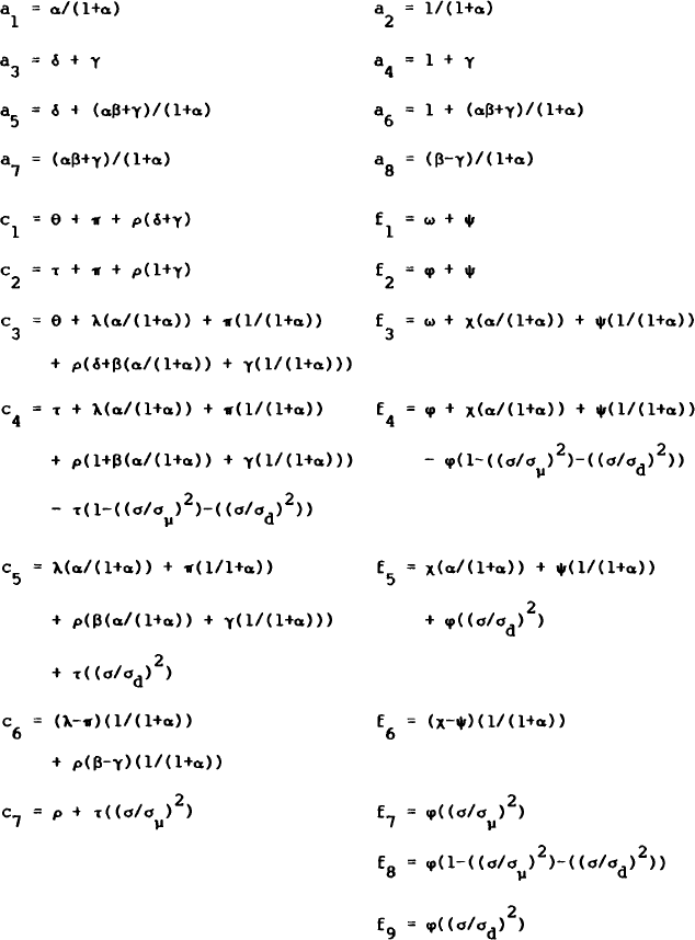
The elements of the coefficients matrices for equations (20) and (21) are

It only remains to show that σ² solves the quadratic in equations (26) and (27). This quadratic is

by equation (A6).

Footnote

From the coefficients of the quadratic in A(6), the product of the roots must be negative. This solution thus yields a unique, positive (real) value for σ². [28]