Research Discussion Paper – RDP 2023-04 Can We Use High-frequency Yield Data to Better Understand the Effects of Monetary Policy and Its Communication? Yes and No!
1. Introduction
To set monetary policy appropriately, it is important for the central bank to understand how monetary policy affects the economy. However, it can be difficult to quantitatively assess the effects of monetary policy. One reason is that monetary policy is not set randomly, but rather in response to expected future economic outcomes. For instance, if the central bank forecasts that inflation and activity are going to increase, it will tend to raise rates to keep inflation from rising too far. As such, it could look like inflation is rising in response to higher interest rates, but in fact interest rates are responding to future (expected) inflation: the relationship is endogenous. A second complicating factor is that central banks not only affect the economy by changing current short-term interest rates, but also through their communication about current and potential future policy. However, quantifying the nature and effects of communication is difficult. Moreover, ‘unconventional’ policies such as the yield curve targeting and bond purchase programs used during the COVID-19 pandemic work by affecting longer-term interest rates and expectations, and not just current short-term interest rates.
To get around the first issue, economists often try to identify monetary policy ‘shocks’. These are ‘exogenous’ changes in policy that are unrelated to current and expected economic conditions. As such, these shocks should give a cleaner read of the causal effects of monetary policy on the economy compared to simply looking at rate changes. There is a large literature trying to identify policy shocks, and to quantify their effects, using various approaches (see Section 2 and Ramey (2016) for more details). This includes several papers looking at the Australian economy, including work by Bishop and Tulip (2017), Beckers (2020) and Hartigan and Morley (2020).
To get around the second issue, more recent work has begun incorporating information about longer-term interest rates when constructing measures of monetary policy shocks. In particular, the recent literature has looked at high-frequency changes in interest rates with different maturities just before and after a policy announcement. These high-frequency changes are interpreted as shocks to current and expected future interest rates as they are above and beyond what market participants expected based on their understanding of systematic monetary policy and the available information. This allows for a more holistic examination of the different facets of monetary policy and its communication, and how these different facets affect the economy.
In this paper we adopt one such approach put forward by Kaminska, Mumtaz and Šustek (2021) (KMS) and apply it to the Australian data. The approach involves combining high-frequency data on changes in yields around policy announcements with an affine term structure model (ATSM), which decomposes the yields into expected future interest rates and term premia. This allows us to further decompose monetary policy shocks into three different components: (i) shocks to the current short-term policy rate – ‘Action’ shocks; (ii) shocks to the expected path of rates due to communication about future conditions or policy intentions – ‘Path’ shocks; and (iii) changes in required term premia due, for example, to the effect of communication on uncertainty or, in the case of unconventional policy, on the supply of government bonds – ‘Premia’ shocks. We then examine the effects of these different shocks on the Australian economy, using them as instruments in a proxy structural vector autoregression (SVAR).
This approach offers three key advantages over previous work. First, as each facet of policy could affect the economy differently, this decomposition potentially allows us to get a cleaner read on each one, rather than lumping them all together. Second, the approach allows us to try to quantify the effects of the RBA's communication about the outlook for rates and the economy. And third, we can apply this approach to COVID-19-era monetary policy to better understand the channels through which it affected the economy.
We apply this approach to monetary policy announcements, while also considering other events, such as speeches, release of Board minutes, and release of the Statement on Monetary Policy. This makes our paper the first to identify the macroeconomic effects of monetary policy shocks around a broad set of different monetary policy-related announcements in Australia.
To preview the results, we find that the KMS approach provides an intuitive lens through which to examine monetary policy and its communication. It allows us to understand how policy and its communication affected expectations for rates and risk during certain historical periods, and more generally. For example:
- During the mid-2010s, Path shocks tended to raise expectations about future interest rates as the RBA communicated concerns around risks in the housing market.
- Monetary policy announcements are more likely to be associated with increased term premia during periods of uncertainty, like the global financial crisis (GFC).
- Changes in term premia were the key channel through which policy affected interest rates during the COVID-19 era, while changes in expected future interest rates played a smaller role. This contrasts with pre-COVID-19 policy announcements, which mainly affected expected interest rates. This finding is similar to overseas findings comparing conventional and non-conventional policy periods (e.g. Kaminska and Mumtaz 2022).
- Speeches and other events mainly contain information about future interest rates, though on average they have a much smaller effect on yields compared to policy announcements.
We also find some evidence that shocks to the path of interest rates were predictable based on information at the time. This suggests that markets systematically misunderstand how the RBA reacts to data, potentially because they are learning about this reaction function over time. This highlights the importance of clear communication.
Regarding the effects of monetary policy on the macroeconomy, the KMS high-frequency approach provides broadly similar estimates of the effects of monetary policy to earlier papers in the literature. Positive shocks to current policy (Action shocks) are associated with an appreciation of the exchange rate and an eventual rise in unemployment. These effects are similar to those found using other simpler approaches, such as using high-frequency yield changes directly, including the fact that the ‘price puzzle’ is still evident, with Action shocks tending to precede higher inflation. In addition, the macroeconomic effects of both Path and Premia shocks turn out to be imprecisely estimated. As such, the approach adds little to our understanding of the quantitative effects of monetary policy on the macroeconomy.
In the context of the broader literature, we also find evidence that the specification of the ATSM can have substantial effects on the estimated shocks. This is consistent with other papers, such as Kim and Orphanides (2012), but is important to highlight in the context of interpreting the effects of monetary policy. In particular, if we follow KMS and use statistical methods to adjust the ATSM, rather than augmenting it with surveys, the approach attributes a much larger share of shocks to changes in the path of interest rates, rather than premia. In turn, this can influence the interpretation of the effects of Path and Premia shocks.
The rest of the paper proceeds as follows. Section 2 provides an overview of the literature on monetary policy shocks. Section 3 describes the KMS approach and shows the corresponding decomposition of yield curve changes. Section 4 examines the effects of the different identified shocks over the pre-COVID-19 period. Section 5 applies the KMS approach to COVID-19-era policy, and finally Section 6 concludes.
2. Related Literature
Our paper relates to the large literature that tries to identify monetary policy ‘shocks’ – movements unrelated to economic conditions (see Ramey (2016) for detailed reviews of the literature). One of the most common approaches to identifying shocks and their effects is to use SVARs along with some identifying restrictions about the timing, magnitude or direction of the effects that shocks have on other economic variables. Numerous papers have applied these approaches to Australian data (e.g. Berkelmens 2005; Beechey and Österholm 2008; Lawson and Rees 2008; Jääskelä and Jennings 2010; Jääskelä and Smith 2011; Read 2022). A common finding in the Australian literature is that while increases in interest rates tend to be contractionary for the economy, they also tend to be associated with increases in inflation: the so-called ‘price puzzle’.
More recently, papers have tried to identify monetary policy shocks using other types of data. For example, Romer and Romer (2004) estimate how the Federal Reserve sets interest rates based on current and expected future conditions, and then use this to identify movements that appear unrelated to these conditions. Bishop and Tulip (2017) and Beckers (2020) both apply this approach to the Australian data. The latter, by also incorporating indicators of financial conditions into the reaction function, is able to overturn the price puzzle. In a somewhat similar vein, some papers have tried to account for this additional information by increasing the information set included in the SVAR (Gambetti 2021). For example, Hartigan and Morley (2020) are able to overturn the price puzzle by including factors extracted from a large macro dataset into the VAR.
Our paper relates more directly to a more recent stream of the literature that has used high-frequency changes in interest rates around policy or other central bank announcements. Using these ‘surprises’ as monetary policy shocks relies on three assumptions:
- during the short window under examination the announcement is the only economic news, so any change can be fully attributed to the announcement.
- the market has priced in all information about future economic conditions, and so the surprise reflects only information about monetary policy that is unrelated to economic outcomes.
- the market understands how the central bank will react to the available information.
One key advantage of the high-frequency approach is that it allows us to incorporate information from across the yield curve. This opens up the possibility of understanding not only the transmission of monetary policy through changes in the current policy rate, but also how policy and its communication can affect the economy by changing expectations about future rates, as well as people's views about risks and therefore the premia they require to invest.
Early papers in this literature focus on a single short-term interest rate to identify shocks to current rates – Action shocks (Kuttner 2001; Gürkaynak, Sack and Swanson 2005b). Gürkaynak, Sack and Swanson (2005a) extend this analysis while focusing on shocks to both current and future expected rates – Action and Path shocks – by looking at high-frequency changes in interest rates with maturities up to one year.
More recent papers on identification using high-frequency policy surprises point out that the second assumption noted above is likely to be violated in many cases, and that the surprises are likely to combine true policy shocks with additional information about the state of the economy – an information shock. In particular, an unexpected increase in the policy rate could indicate that the central bank expects economic conditions to improve, reflecting additional information held by the central bank and not available to the market. This reintroduces the standard endogeneity issue that shocks are meant to avoid. Jarockinski and Karadi (2020) and Miranda-Agrippino and Ricco (2021) show that ignoring these information shocks leads to biased estimates of the effects of monetary policy. He (2021) explores information shocks in the Australian context, finding some evidence that speeches contain such information, but little evidence for other communication.
An alternative explanation of the information shocks is the ‘Fed response to news channel’ proposed by Bauer and Swanson (2021, 2022). They show that their empirical results are consistent with incoming, publicly available economic news causing the Fed to change monetary policy, but the private sector systematically underestimating the Fed's response. This leads to a violation of the third assumption. They provide substantial new evidence that distinguishes between news and the response to news channels. The evidence strongly favours the response to news channel. They also outline a model where market participants learn about the Fed's reaction function, which can explain systematic misunderstanding of the Fed's response.
Another recent debate in the literature revolves around the role of term premia and financial conditions in the transmission of monetary policy shocks. Using high-frequency changes in interest rates around announcements for the United States, Gertler and Karadi (2015) find that monetary policy shocks transmit through the economy largely by affecting term premia, with expected future interest rates left almost unaffected. To this end, they highlight the importance of including financial variables in models to capture the transmission of monetary policy through the credit markets.[1] Consistent with this, Caldara and Herbst (2019) find that US monetary policy has a strong and systematic response to financial conditions, underlining the importance of including financial variables such as credit spreads in the VAR or when constructing shock measures using the Romer and Romer (2004) approach.
Gertler and Karadi's (2015) finding that monetary policy transmits to the economy almost exclusively through changes in term premia presents a challenge to theoretical models used for monetary policy analysis. This, alongside the earlier noted debate around information shocks, motivated KMS to revisit the relevance of Action, Path and Premia shocks using a more structural approach.
Specifically, KMS apply an ATSM to high-frequency data on changes in the yield curve around Fed policy announcements. This allows them to decompose these changes into changes in expected rates and term premia. Using additional restrictions in a second step, they further decompose these surprises into three different facets of monetary policy and its communication: changing current short-term rates – Actions shocks; changes in the expected path of rates – Path shocks; and changes in term premia or uncertainty – Premia shocks. They then study the macroeconomic effects of the different facets of monetary policy using a local projections model. Overall, they find that Action shocks affect the economy like textbook monetary policy shocks. Path shocks appear to capture signalling about future economic conditions, while Premia shocks are hard to interpret, but have some hallmarks of uncertainty shocks.
Our paper also relates to the literature on ATSMs. In particular, several papers have highlighted that ATSMs tend to produce unreasonably stable estimates of expected rates in the far future. This reflects small-sample biases in these models. Some papers have suggested using statistical approaches to address this bias (e.g. Malik and Meldrum 2016), as used in KMS. In contrast, other papers have argued for the incorporation of surveys to provide additional information on the expected path of short-term interest rates (e.g. Kim and Orphanides 2012; Guimarães 2016). As we show in Appendices A and B, the choice of approach can affect the identified shocks in the KMS framework and therefore alter the interpretation of the shocks.
3. Documenting Shock Measures Pre-COVID-19
As discussed above, KMS suggest a new approach to identifying monetary policy shocks using high-frequency data that is able to separate out the effects of action, signalling/forward guidance, and effect on term premia. Specifically, KMS suggest a three-step approach to constructing more interpretable monetary policy shocks:
- Gather high-frequency measures of surprise yield changes.
- Decompose changes in yields into changes in expected policy rates and changes in premia.
- ‘Reshape’ these changes in expected rates and premia to capture shocks to the current policy rate, to the expected future path of policy rates, and to premia or uncertainty.
3.1 Gathering high-frequency yield changes
As noted above, the KMS approach builds off the high-frequency identification literature, taking changes in yields over tight windows around events as exogenous monetary policy shocks. For this, we use data on overnight indexed swaps (OIS) at fixed maturities of 1 week, 1 to 6 months, 9 months, and 12 months, as well as yields on all outstanding nominal Australian Government securities with at least 1 year to maturity. These are measured in a reasonably tight window of 30 minutes before the relevant event, and 90 minutes after. We use these data to fit a zero-coupon yield curve just before and after the announcement, following the approach of Finlay and Olivan (2012).
Our main focus is on monetary policy announcements, which is consistent with much of the literature. We collect data on meetings covering the period from 2002 to 2019.
We also consider the broader set of events examined in He (2021), though we only incorporate data from 2006 to 2019 (as earlier data were not available). This includes speeches, release of the Board minutes, and release of the Statement on Monetary Policy. Considering these extra events not only broadens our information set in general, but may also be particularly useful in identifying shocks to the path of expected interest rates if these longer-form releases provide a more detailed assessment of the likely path for interest rates.
Table 1 provides some statistics on these changes. Variation in yields tends to be higher on monetary policy announcement days, particularly for shorter maturities, with much of the variation occurring during the tight event window. On average across the sample, other event days look fairly similar to the full sample, with the events themselves being associated with relatively minimal variation in yields. This is consistent with the findings in He (2021), though as he notes and we discuss below, some have had larger effects, particularly around the GFC.
| 1-year | 3-year | 5-year | 10-year | Observations | |
|---|---|---|---|---|---|
| Daily change | |||||
| Full sample | 0.033 | 0.043 | 0.044 | 0.046 | 3,714 |
| Monetary policy announcement day | 0.050 | 0.051 | 0.051 | 0.047 | 199 |
| Other event day | 0.029 | 0.042 | 0.042 | 0.042 | 523 |
| Change during window around announcements | |||||
| Monetary policy announcement window | 0.035 | 0.039 | 0.031 | 0.023 | 199 |
| Other event window | 0.013 | 0.018 | 0.015 | 0.015 | 523 |
| Sources: Authors' calculations; RBA; Refinitiv; Yieldbroker | |||||
3.2 Decomposing yield curve changes into changes in expected rates and premia
Following KMS, we decompose changes in the yield curve into changes in the expected path of interest rates and changes in premia by employing a standard ATSM, which is designed to model the future path of interest rates and premia based on data on yields. Our ATSM differs slightly from KMS (for details see Appendix A). First, we use a slightly different estimation procedure, suggested by Adrian, Crump and Moench (2013). But more importantly, we incorporate surveys into the model to avoid small sample biases, similar to Kim and Orphanides (2012) and Guimarães (2016), rather than using statistical techniques as in KMS. As discussed in Appendix A, this leads to a more plausible path for expected interest rates and term premia. It also affects what the model assigns as Path and Premia shocks, affecting our estimates of the effects of these shocks.
Having estimated the model parameters, we can then apply the ATSM to look at the estimated path of interest rates and term premia, before and after monetary policy announcements or other events.[2] For example, Figures 1 and 2 show the yields, expected policy rates and premia just before and after the May 2016 monetary policy announcement where a 25 basis point cut in the cash rate to 1.75 per cent was announced. Yields fell after the announcement with much of the decline reflecting lower current and expected policy rates. Premia also declined, potentially suggesting some decline in uncertainty about future rates.
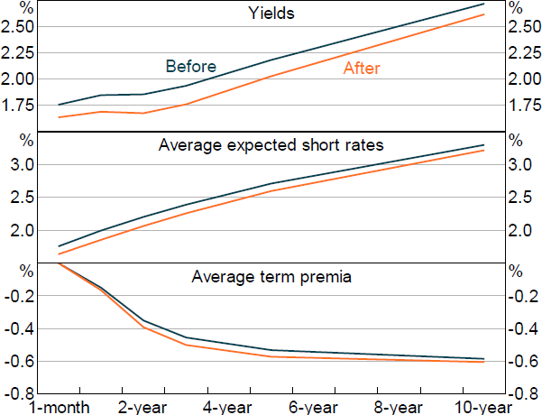
Note: Before is 30 minutes before monetary policy announcement, after is 90 minutes after monetary policy announcement.
Sources: Authors' calculations; Refinitiv; Yieldbroker
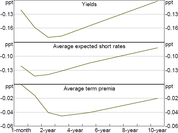
Sources: Authors' calculations; Refinitiv; Yieldbroker
Figure 3 summarises these changes over time at a few points on the yield curve. For monetary policy announcements, changes in expected policy rates tend to be the most important aspect of yield changes, even at longer horizons. But changes in term premia can be quite important as well. For example, premia spiked around policy announcements during the GFC in late 2008, offsetting some of the effects that lower rate expectations had in lowering longer-term yields. Focusing on other events, the figure also shows that while the average effect of these events is smaller, during certain periods these events have had sizable effects on yields, indicating that they can potentially provide useful extra information on monetary policy shocks.
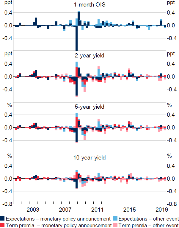
Note: Quarterly sum.
It is interesting to compare these results to an average day in the sample, as this can provide a sense of whether expected rates play a relatively larger role on monetary policy event days. To consider this, we run the ATSM over daily changes in yields across all days in the sample period (from 2002 to 2019). Perhaps unsurprisingly, on days with monetary policy announcements a far larger share of variation in yields reflects changes in expected interest rates compared with an average day (Table 2).
When we focus on non-policy announcements (e.g. speeches), changes in expected rates also play a larger role than premia in driving variation in yields, though typically not to the same extent as around monetary policy announcements. So while these other events primarily contain information about future interest rates, the composition of information released during these events is more skewed towards uncertainty or risk around the path of rates than in monetary policy announcements.
| 1-year | 3-year | 5-year | 10-year | |
|---|---|---|---|---|
| Daily change | ||||
| Full sample | 58 | 47 | 35 | 14 |
| Monetary policy announcement day | 72 | 59 | 50 | 25 |
| Other event day | 64 | 51 | 49 | 30 |
| Change during window around announcement | ||||
| Monetary policy announcement window | 95 | 79 | 75 | 58 |
| Other event window | 72 | 49 | 49 | 31 |
|
Sources: Authors' calculations; RBA; Refinitiv; Yieldbroker |
||||
3.3 Decomposing yield curve changes into changes in Action, Path and Premia shocks
While the above decomposition provides some useful extra information, it still doesn't fully differentiate between the different facets of monetary policy. For example, in the May 2016 announcement did the fall in the average expected policy rate over the next two years reflect the cut in the cash rate, or did it reflect forward guidance or signalling about the state of the economy and rates in the future? Equally, how much of the change in premia is directly related to changes in expected interest rates, which could, in turn, affect investors' views of economic conditions and therefore required term premia, and how much reflected reduced uncertainty about the future as a result of the central bank's communications?
To better understand these different facets of policy, KMS suggest adjusting the above decomposition to capture three distinct and more interpretable shocks:
- Action shocks: changes in expected policy rates flowing from changes in the current policy rate.
- Path shocks: changes in the expected path of policy rates unrelated to changes in the current policy rate (e.g. due to forward guidance or signaling).
- Premia shocks: changes in term premia unrelated to changes in policy rate expectations.
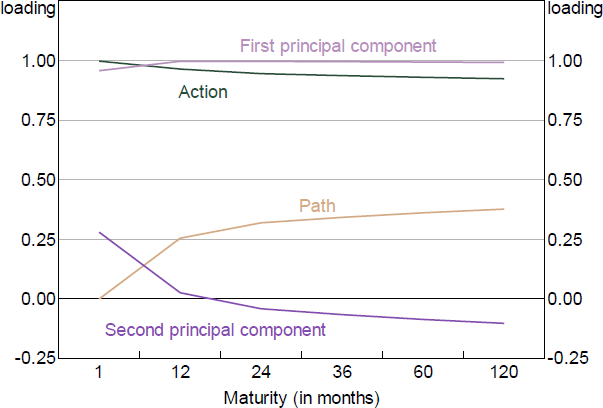
The Action and Path shocks are constructed by taking the first two principal components of changes in expected rates across the curve (i.e. ‘factors’), which summarise the changes, and transforming them so they have a cleaner interpretation. We rotate the factors such that one has no loading on the short-term interest rate: the Path shock. The other is allowed to load on the short rate: the Action shock. This is similar to the approach taken by Gürkaynak et al (2005a), but they apply it to the raw yield curve rather than first removing term premia.[3]
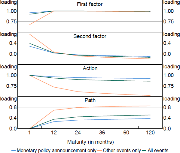
Focusing on policy announcement days, the factor loadings end up looking similar to a ‘level’ and ‘slope’ factor, which is a common finding when taking principal components of a yield curve (e.g. Hambur and Finlay (2018); Figure 4).[4] Action shocks lead to a fairly consistent increase in expected rates across the curve. Path shocks by construction have no effect on current rates, but larger effects on future interest rates, so lead to a steeper yield curve (all else equal).
To construct the Premia shock we compute the residual from a regression of the term premia changes on the above factors, which removes the influence of expected rate changes. We then take the first principal component of these residuals to summarise the changes across all maturities. KMS take the additional step of rotating the term premia so that it does not load on short-term premia, similar to the adjustment made to construct the Path factor. We experimented with this approach and it does not substantially change the results, but does lower the explanatory power of the Premia shocks.
Figure 5 shows the contribution of these different facets of monetary policy shocks to yields over time, focusing on monetary policy announcements. Much of the variation in yields across the curve reflects current policy actions (~65 per cent), and these shocks show a reasonable correlation with the measures proposed in Beckers (2020): around 0.5.[5] Changes in the expected path also play an important role (~20 per cent), while changes in uncertainty/premia account for only a small share (~10 per cent).[6]
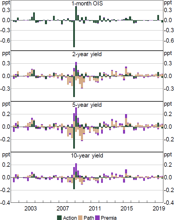
Notes: Decomposition based on regression of yield changes on shocks. Residuals excluded. Quarterly sum.
Similar to the above findings, the dominance of the Action shock seems to be particularly evident on monetary policy announcement days. If we run the model over all days from 2002 to 2019 (and enforce the same factor loadings), the Path shock accounts for around 1.5 times as much variation in yields as the Action shock across different maturities.[7] In contrast, on announcement days the two play a broadly similar role (and the Action shock is more important within the window). Similarly, focusing on other event days the Action shock accounts for only around 15 per cent of variation, compared with 60 per cent for the Path and 20 per cent for the Premia shock.[8] This suggests that monetary policy announcements are unique in containing mainly information related to interest rates in the immediate future (perhaps unsurprisingly).
Even if Path and Premia shocks are relatively less important overall in policy announcement events, they have played crucial roles at different stages, particularly for medium-to-longer-term yields. For example, Path shocks consistently lowered medium-term yields during the early stages of the GFC in early and mid-2008. To understand this, we use simple text analysis of the policy announcement. We find that the negative path shocks coincided with increased references to softening credit and economic conditions, volatile overseas outcomes, and economic risks, as evident from the increase in the number of references to risk in the monetary policy announcements (Figure 6).[9]
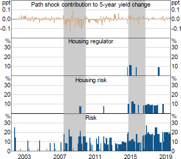
Notes: Housing words include: dwelling prices, housing credit, housing market, housing conditions and household debt. Risk words include: downside risk, concern(s) and risk(s). Regulator words include: regulator(s) and APRA. Abating words include: eased, declining, decline(s), easing, fall(s) and abate. Housing regulator includes a housing word and a regulator word. Housing risk includes a housing word and a risk word. All groups exclude any abating words.
Sources: Authors' calculations; RBA
Similarly, Path shocks seem to have consistently raised short- to medium-term yields during the mid-2010s. This was also evident for other events (see Figure B2). One potential explanation could be that increased references to housing prices and risks caused markets to adjust their expectations for future policy rates higher. To consider this, we again use simple text analysis to look for references to risks in housing markets or to the regulator (with no offsetting word) in monetary policy announcements. As shown in Figure 6, references to these risks have tended to coincide with positive path shocks. While this finding is by no means causal and conclusive, it does provide some evidence that the shocks are able to parse some of the relevant information being communicated about the future path of interest rates.
Meanwhile Premia shocks appear to be related to monetary policy uncertainty. There were large Premia shocks around monetary policy announcements during the GFC, a period of heightened uncertainty. Moreover, there is a reasonable positive correlation between various proxies for monetary policy uncertainty and Premia shocks. For example, forecaster disagreement regarding the future cash rate as measured in the RBA Survey of Market Economists, a proxy for uncertainty, has a moderate correlation with the size of the Premia shocks in that quarter (Figure 7, top panel). This relationship is not present when looking at the Action or Path shocks, and does not simply reflect the GFC period. Similarly, there is a moderate correlation between the (conditional) volatility of the 3-month OIS and the Premia shock in a given month.[10]
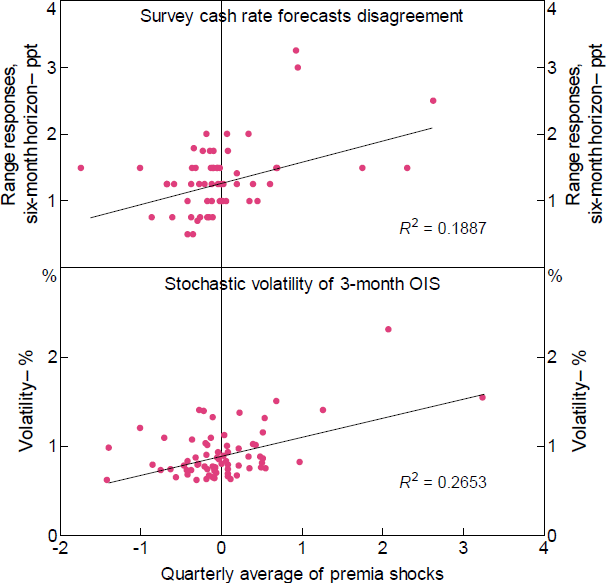
Sources: Authors' calculations; RBA
Finally, one natural question about these shocks is whether they are truly exogenous and unpredictable. Several papers have argued that high-frequency shocks can still be endogenous if the central bank has some additional economic information that it communicates, or if market participants misunderstand the central bank's responses to data (Nakamura and Steinsson 2018; Bauer and Swanson 2021, 2022). The former will naturally be captured in the Path shocks as this additional information about future outcomes should influence expected future interest rates. Separating this out, and being able to look at this aspect versus the effect of current actions is a key benefit of the KMS approach. The latter remains a cause for concern and so we explore it below.
To understand whether market participants systematically misinterpret the RBA's response to incoming data, we consider whether they could have ‘predicted’ the shocks using available data. Specifically, we regress each shock on various measures of economic and credit conditions which include the following: changes in the unemployment rate and (log) employment over the preceding twelve months, and three-month changes in the (log) TWI, money market spread (3-month BBSW less OIS), the US commercial paper spread, the second principal component of the yield curve (strongly related to its slope), (log) commodity prices, (log) ASX 200, the US VIX and the US corporate bond spread (BAA). These variables are motivated by Bauer and Swanson (2021, 2022) and Beckers (2020). The regression is run separately while including and excluding the GFC period, to allow for the fact that the relationships may have changed during this period.[11]
We find that these factors explain around 20 per cent of the variation in Action shocks, 25 per cent of the variation in Path shocks and 15 per cent of the variation in Premia shocks when the GFC is included in the sample. If we exclude the GFC, the share for the Action shocks declines substantially but remains the same for the other two components. This suggests that while the Action shocks are truly unpredictable, with the benefit of hindsight, market participants may have been able to predict the other shocks. It also suggests that the nature of what is being identified as a shock during the GFC could differ from the rest of the sample, potentially reflecting less efficient price discovery and incorporation of information during this volatile period.
How can we explain this predictability and the apparent systematic misunderstanding of the RBA's reaction function, at least with respect to the future stance of policy? One explanation is that markets learn about the reaction function over time (Bauer and Swanson 2021, 2022). Relatedly, the reaction function could change over time, and agents may be slow to learn about those changes. This could explain the autocorrelation observed in the Path shocks, which is removed once we orthogonalise the shocks with respect to available data. In either case, the results speak to the importance of effectively communicating the RBA's reaction function.
Interestingly, if we focus on the other events alone, the degree of predictability is far lower, in the region of 5 to 10 per cent. This suggests that these events contain relatively more exogenous information.
In terms of using these shocks as instruments for monetary policy, the predictability of the Path and Premia shocks indicates that they are unlikely to be a valid instrument as they may be correlated with other structural shocks or expected future economic outcomes. That said, the direction of the bias will be less clear, and will be dependent on whether participants over or underweight certain variables. Rather than exploring deeply the nature of the systematic error, we simply consider the macroeconomic effects of the shocks with and without the orthogonalisation step in the next section.
4. The Effects of Monetary Policy Shocks
The above section highlights that these new measures of monetary policy shocks contain relevant information about monetary policy and its communication. Given they seem to capture different facets of monetary policy, they may have different macroeconomic effects, and therefore this decomposition could potentially provide useful quantitative estimates of how monetary policy and its communication affect the macroeconomy.
To consider this we use an instrumental-variable structural vector autoregression (IV-SVAR) approach. This approach was pioneered by Stock (2008), Stock and Watson (2012, 2018) and Mertens and Ravn (2013). The idea behind this approach is to use instruments (in our case policy surprises as discussed above) to identify (different facets of) monetary policy shocks from a reduced form VAR.
More precisely, we consider the following proxy SVAR model (see also Doko Tchatoka and Haque (2021))
where Yt is an n×1 vector of endogenous variables, ut is an n×1 vector of reduced-form innovations, p is the number of lags, and are n×n matrices of unknown coefficients. The reduced-form innovations are related to the structural shocks as follows:
where A0 is an n×n non-singular matrix and the structural shocks are assumed to be serially and mutually uncorrelated and satisfy the following:
The variance-covariance matrix of the reduced-form innovations is given by
Yt has a structural moving average (MA) representation
where B = (B1, B2,...,Bp) and Ck (B) highlight the dependence of the MA coefficients on the autoregressive coefficients in B, that is
with C0(B) = In and Bm = 0 for m > p (e.g. Montiel Olea, Stock and Watson 2021).
The structural impulse response function is the response of Yi,t+k to a one-unit change in , which is given by
where ei and ej denote the ith and jth columns of the identity matrix In, respectively.
Following Gertler and Karadi (2015), we identify the policy shock using an external instrument. Let zt denote an external instrument and be an (n–1)×1 vector of structural shocks other than the monetary policy shock. The key identification assumption in the external instrument approach is that zt is correlated with but uncorrelated with . Stock and Watson (2018) and Montiel Olea et al (2021) show that if this identifying assumption holds, then one can identify the structural shock of interest.
Our baseline VAR is estimated (using ordinary least squares) at a monthly frequency. The variables included in the IV-SVAR are: unemployment rate, (log) retail sales, (log) housing prices, (log) dwelling approvals, the mortgage spread (variable owner-occupier rate less cash rate; adjusted for a break around the GFC), the (log) nominal TWI, and the first two principal components of the yield curve. The VAR is estimated over the sample from January 1994 to December 2019, while the high-frequency surprises that are used to identify the structural policy shocks only begin in 2002. We examine the effect of each of the surprise components one-by-one, using them as instruments for the yield curve factors. Confidence bands are constructed using a wild bootstrap.[12]
Many papers incorporate specific interest rates, such as the cash rate, or other short-term interest rates. Given some of our shocks directly affect longer-term rates and not short-term rates, we also need to incorporate longer-term rates. Rather than choosing yields of certain maturities, we use the first two principal components of the yield curve in the VAR, similar to KMS. This allows us to flexibly account for the effect of the shocks, rather than taking a stand on the most relevant maturity, although it does make scaling and interpreting the shocks more challenging. We consider the effect of a shock that leads to a one standard deviation increase in one of the factors. We can then use the factor loadings to estimate the effect on relevant interest rates.
4.1 Monthly VAR
4.1.1 Action shocks
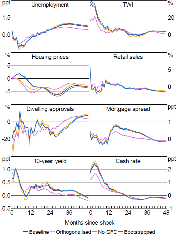
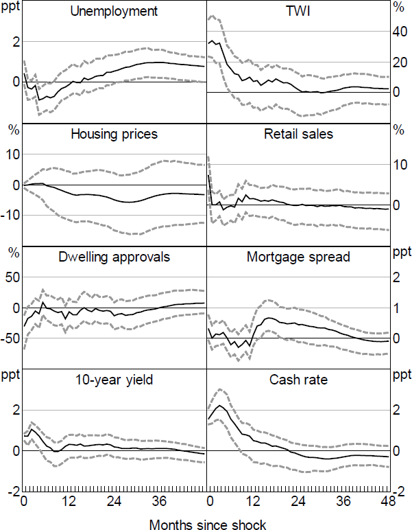
Figure 8 shows the impulse responses from an Action shock focusing on monetary policy announcements. The shock is scaled to lead to a one unit increase in the first principal component of the yield curve, which equates to around a 200 basis point increase in the cash rate. The shock has a robust F-statistic for instrument strength of around 10, which is the level often used to assess instrument strength (Staiger and Stock 1997; Table B1).

Note: Dashed lines denote 90 per cent confidence intervals (bootstrapped).
The responses are largely consistent with what would be expected from a standard contractionary monetary policy shock. Both short- and longer-term interest rates rise, the exchange rate appreciates instantaneously, and the shock leads to an eventual increase in unemployment, while housing prices decline somewhat over time.
Nevertheless, there are some surprising dynamics as unemployment initially declines. Part of this appears to reflect the inclusion of the GFC period, with the extent of the decline tending to be much smaller if this period is removed (Figure B3). Similarly, the response of the TWI is also somewhat larger than would generally be expected but becomes smaller if the GFC period is removed.
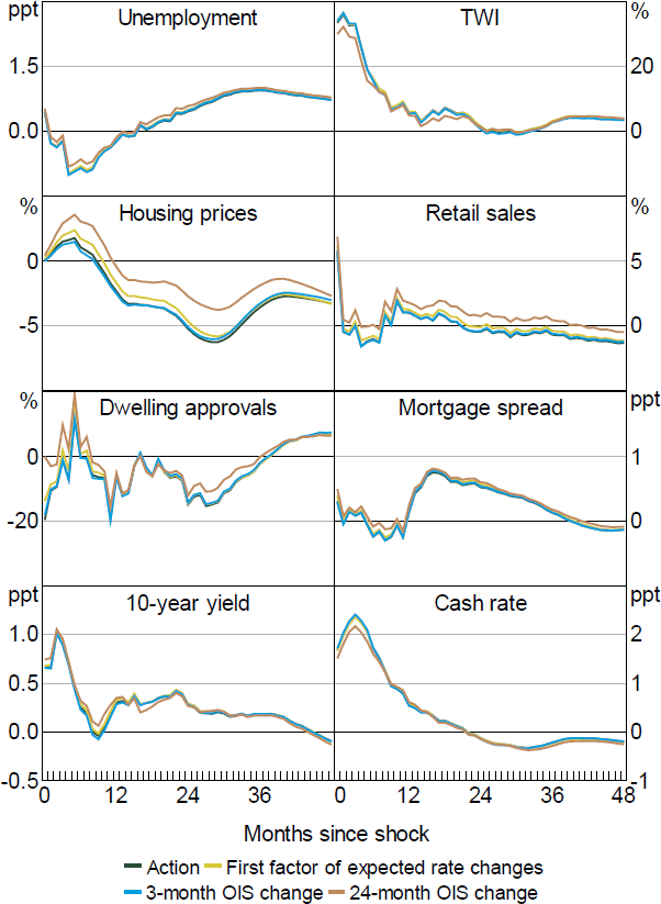
Overall, the results are very similar to those obtained from simpler approaches, such as taking information directly from the yield curve without applying an ATSM. For example, using just the change in the 3-month or 2-year OIS rate around the Board meeting leads to very similar results, as does simply taking the first factor of the change in expected short rates from the ATSM changes without rotating to extract the Action and Path shocks (Figure B6).[13] This provides some initial evidence that suggests that the identified Path and Premia shocks might have a fairly small systematic effect on economic outcomes.
Expanding the information set to include other events has relatively little effect on the results (Figure B7). This is unsurprising given the earlier findings that Action shocks were mainly relevant on policy announcement days.
4.1.2 Path shocks
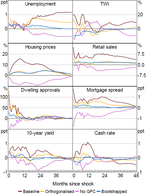
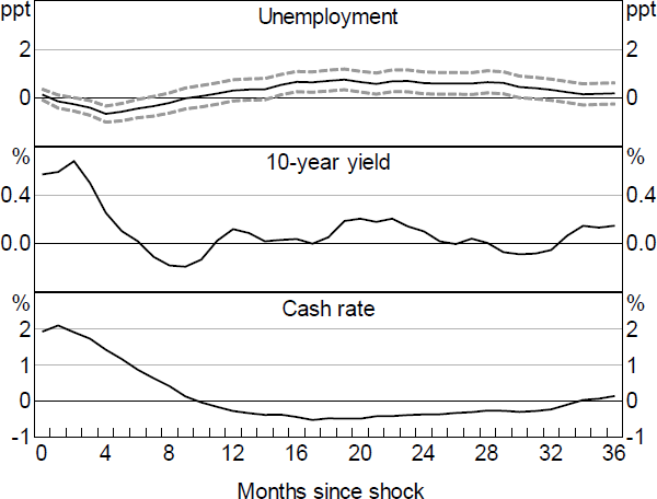
The Path shock appears to be a fairly weak instrument for monetary policy shocks, with a very low F-statistic (Table B1). Accordingly, the effects are imprecisely estimated with large confidence bands and as such Figure 9 only reports the point estimates.[14] Moreover, the responses are not particularly robust to specification changes such as removing the GFC period or orthogonalising the shocks (Figure B4).
Expanding the information set to include the broader set of events does little to change the results, which remain poorly identified with a very low F-statistic (Table B1). This remains the case when we use only the non-monetary policy announcement events.
One explanation for the fact that Path shocks appear not to have significant macroeconomic effects is that policy and other announcements have little to no economic effects via signalling or information channels, unlike in the United States (per KMS). This would be somewhat consistent with He (2021) who finds little evidence of signalling effects in RBA announcements apart from speeches when looking at equity prices using a simpler approach with high-frequency yields.
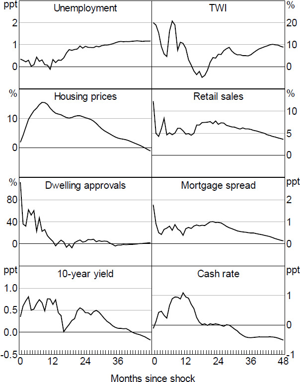
Note: No responses are significant.
Another potential explanation is that Path shocks capture different aspects of the RBA's communication at different points in time. As discussed in Section 3, in the lead up to the GFC the declines in rates appear to signal downside risks to future economic conditions, consistent with standard signalling channels. But in the mid-2010s, the increases in future expected policy rates appear to reflect the RBA indicating that rates may remain elevated due to concerns over potential risks in the housing market, a pure monetary policy shock that would weigh on macroeconomic outcomes. In both cases the Path shocks would be associated with weaker economic conditions, but one set was positive and the other was negative, so the average effect of Path shocks may net out when used in the SVAR.
4.1.3 Premia shocks
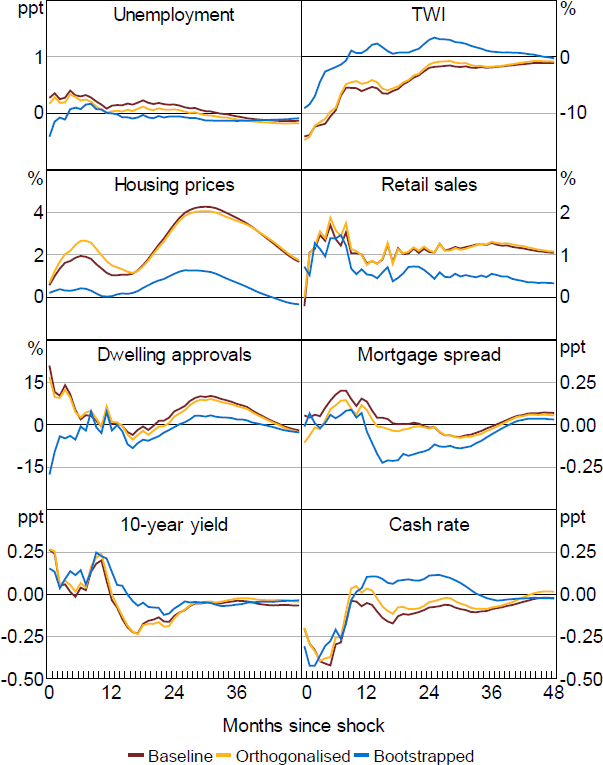
As in KMS, the responses to Premia shocks are difficult to interpret and do not conform to a standard view of the impact of uncertainty (Figure 10). Moreover, the impulse responses are highly sensitive to the inclusion of the GFC period, and are imprecisely estimated, consistent with Premia shocks being a weak instrument for changes in the yield curve, with a very low F-statistic (Table B1; Figure B5).
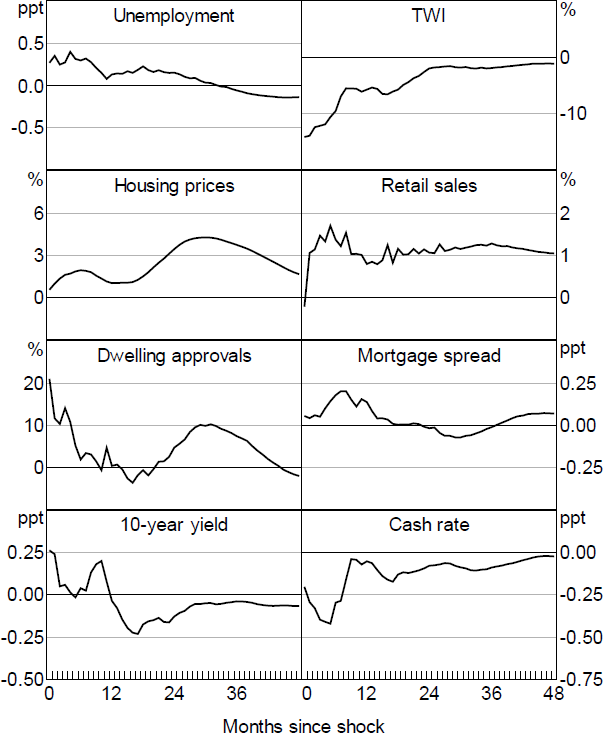
Note: No responses are significant.
Again, expanding the information set does little to change the results. The Premia shocks still represent weak instruments, with poorly identified responses.
4.2 Quarterly VAR
As the policy shocks are constructed at a monthly frequency, we use a monthly VAR for the baseline analysis. To consider whether these shocks are able to overturn the well-known price puzzle, we also estimate a quarterly VAR. The variables are largely the same, however, we include the log trimmed mean CPI in the model and replace retail sales with log GDP and the nominal TWI with the real TWI. We sum the shocks in each quarter to get a quarterly shock series.
Figure 11 shows the results for the Action shock. Overall, the responses of most variables are similar to the monthly results. However, inflation rises following the shock, suggesting that the Action shock still contains some endogenous component. Orthogonalising the shocks does little to change this result, nor does removing the GFC period. This suggest that the high-frequency identification approach itself is unable to solve the price puzzle.
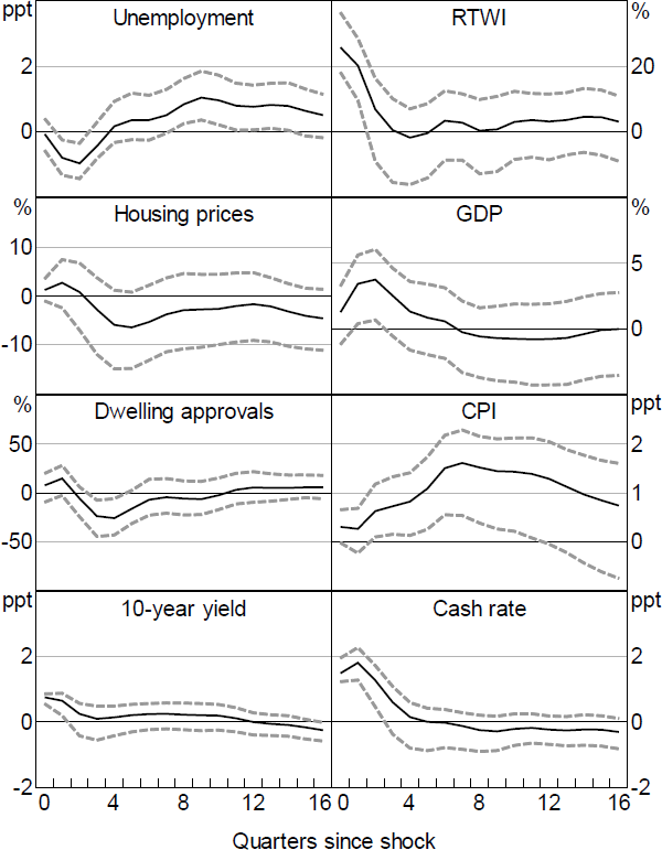
Note: Dashed lines denote 90 per cent confidence intervals (bootstrapped).
4.3 Robustness
We perform a number of checks to assess the robustness of the results for both the monthly and quarterly VAR. As we note above, we consider removing the GFC period. The main systematic difference is to the results for the Action shock, with the surprising initial decline in unemployment being less significant this time.
As noted above, we also consider orthogonalising the shocks to remove any systematic relationship with variables that were known at the time, removing what Bauer and Swansson (2022) refer to as the ‘Fed response to news’ effect. Doing so has little implication for the Action shocks but leads to much more muted responses for the Path shocks. This is consistent with the interpretation of these shocks as capturing RBA signals about future outcomes that are based on available news on recent outcomes, with markets systematically underappreciating this additional news.
In terms of the price puzzle, our results may reflect an information sufficiency issue in small-scale SVARs (e.g. Gambetti 2021). For example, Hartigan and Morley (2020) find this information deficiency to be relevant for Australia and resolve the price puzzle using recursive identification in a factor augmented VAR (FAVAR) with two factors extracted from a large macro dataset. Accordingly, we incorporate the macro factors from Hartigan and Morley to increase the information set in our estimated VAR. However, the effects of the Action shock remain largely unchanged with the price puzzle still remaining unresolved in our high-frequency identification setting.
As an alternative approach to the IV-SVAR we also consider a Bayesian local projections model, as in KMS. The results are generally quite similar to our baseline results, with the Action shock leading to an economic contraction, while the other shocks lead to poorly identified economic responses (Figure B8). This helps to address concerns around our choice of bootstrapping methods (see above).
The main other robustness check we consider is changing the ATSM. In particular, rather than incorporating surveys into the ATSM, we account for the small-sample bias using bootstrapping, similar to the statistical approach taken in KMS. Taking this approach leads to very similar estimated effects for the Action shocks (Figure B3). The main differences are evident in the Path and Premia shocks with the responses tending to be more muted (Figures B4 and B5).
Our finding that the specification of the ATSM matters for the estimation results is not surprising. As discussed in Appendix A, the choice of small-sample adjustment can lead to very different estimated paths for future expected interest rates and term premia, with the survey model providing a more sensible account of history. This suggests that in adopting the KMS approach, it is important to think about the specification of the ATSM, as it can have substantial implications for what the model interprets as Path and Premia shocks. While this doesn't seem to be important in the Australian case, given only the Action shock has macroeconomic effects, it could be more important in other countries.
5. Documenting Shock Measures during the COVID-19 Pandemic
The above analysis shows that while the KMS approach does not seem to add much to our quantitative understanding of the macroeconomic effects of monetary policy shocks in Australia, it is still a potentially useful framework for understanding the multi-faceted nature of monetary policy decisions and their communication.
Such a framework could be particularly useful in trying to interpret the RBA's COVID-19-era policy. The cash rate was reduced to around the effective lower bound, and various unconventional policies were introduced, including a yield curve target and a bond purchase program. Previous work has analysed these programs and their effects on markets in detail, exploiting differential outcomes across different markets and instruments (Finlay, Titkov and Xiang 2022). However, the KMS approach provides another lens through which to examine these policies, decomposing them into effects on expected rates and term premia using a statistical model.
As such, we apply the KMS approach to a number of key dates around the announcement of the RBA's package of support policies, including the yield curve target and the bond purchase program. These are based on the dates examined in Finlay et al (2022). The full list is covered in Table 3.[15]
| Date | Event |
|---|---|
| 16 March 2020 | RBA statement that the it ‘stands ready to purchase Australian government bonds in the secondary market to support the smooth functioning of that market’ |
| 19 March 2020 | RBA announced a package of policy measures |
| 14 September 2020 | Newspaper article (‘RBA and markets out of tune’) |
| 22 September 2020 | Speech by Deputy Governor Debelle |
| 23 September 2020 | Market economist report calling for further policy easing |
| 6 October 2020 | October monetary policy announcement |
| 7 October 2020 | Newspaper article (‘Odds shortened on more easing’) |
| 15 October 2020 | Speech by Governor Lowe |
| 26 October 2020 | Newspaper article (‘RBA to buy bonds’) |
| 3 November 2020 | November monetary policy announcement of bond purchase program |
| 2 February 2021 | First extension of bond purchase program announced |
| 6 July 2021 | Announcement of tapering in bond purchases |
|
Note: Yield change measured as close-to-close. Sources: Finlay et al (2022); RBA |
|
The analysis is similar to the work of Kaminska and Mumtaz (2022), who find that term premia play a larger role in monetary policy shocks in the UK post-quantitative easing period (from 2009 to 2019). However, our analysis differs in a number of ways. First, we focus on a shorter period and a smaller number of specific announcements, more akin to an event study approach. And relatedly, we only focus on the first step of the approach, decomposing rate changes into changes in expected rates and term premia. Given the cash rate was at the effective lower bound for most of the event dates, the further decomposition into ‘Action’, ‘Path’ and ‘Premia’ seems less relevant.
More importantly, our ATSM does not explicitly account for the effective lower bound on interest rates (or asset purchases). Previous work has shown that failing to account for the effective lower bound can lead the ATSM to expect rates to pick up more quickly than the market actually expects (e.g. Andreasen and Meldrum 2013). In turn this will bias down the premia, and therefore may cause us to overstate the role of term premia compared to rate expectations. As such, the result should be thought of as somewhat of an upper bound on the role of premia.
Figure 12 shows the results focusing on the March announcements of the first package. As discussed in Finlay et al (2022), this led to a large decline in yields at the short end of the curve but, on net, a moderate increase in longer-term yields. Our results imply that a decline in expected future interest rates pushed down yields at the short end of the curve, consistent with the market interpreting the announcements as signalling that the cash rate would be kept low for a period, particularly the announcements on 19 March which included an announcement of the yield curve target. The announcement of the yield curve target also coincided with a substantial decline in the premia on yields for 3-year bonds not evident elsewhere on the curve, suggesting that part of the effects of the policy came through this channel. This finding is consistent with Lucca and Wright's (2022) findings for Australia, and more generally with D'Amico and King's (2013) findings of ‘local supply effects’ on targeted maturity bonds for US bond purchases.
Focusing on the long end of the curve, the documented rise in rates seems to have largely reflected increases in premia. As noted by Finlay et al (2022), it is hard to make a strong case that the announcement ‘caused’ premia on longer-term yields to rise, but it does suggest that the announcement did little to lower the premia.
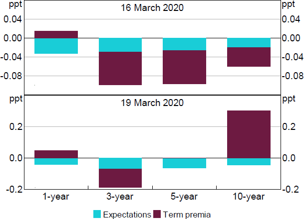
Note: Measured from previous day close to current day close.
Sources: Authors' calculations; RBA
Focusing on the later dates associated with the bond purchase program, we see that much of the effects seem to have come through lower premia, with only a smaller share of the decline reflecting lower expected future rates (Figure 13). This finding is similar to that of Finlay et al (2022) and suggests that the program largely worked through reducing premia. It is broadly consistent with other findings in the literature, though findings on the split between premia and signalling do vary across different unconventional monetary policy programs (e.g. Busetto et al 2022).
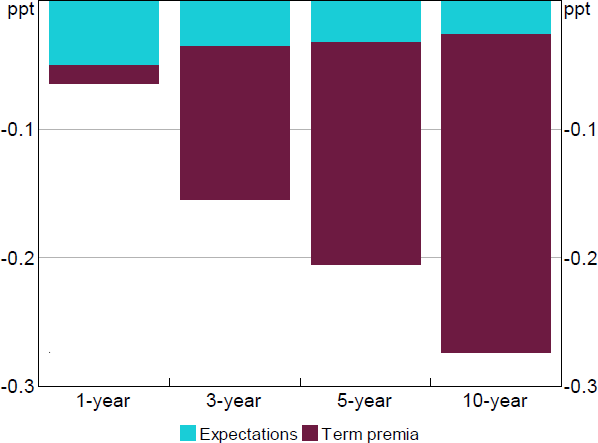
Note: Measured from close of previous day to close of day over each of the dates listed in Table 3, excluding 16 and 19 March 2020 and 6 July 2021.
Sources: Authors' calculations; RBA
More generally, during the COVID-19 period term premia appear to have played a much larger role in the transmission of monetary policy and monetary policy announcements. To see this, Table 4 compares the share of variation in rates accounted for by rate expectations for pre- and during COVID-19 monetary policy announcement dates. This is similar to the findings in Kaminska and Mumtaz (2022) for the United Kingdom. Taken together, the results suggest a much larger role for term premia in the transmission of COVID-19-era policy, consistent with Finlay et al (2022).
| 1-year | 3-year | 5-year | 10-year | |
|---|---|---|---|---|
| Pre-COVID-19 monetary policy announcement | 72 | 59 | 50 | 25 |
| COVID-19 monetary policy announcement(a) | 51 | 22 | 30 | 3 |
|
Note: (a) Removing large change in 10-year term premia on 19 March 2020. Sources: Authors' calculations; RBA |
||||
6. Conclusion
This paper explores a new approach to identifying the effects of monetary policy and its communication in Australia. Following Kaminska, Mumtaz and Šustek (2021), we combine high-frequency data on changes in yields around policy announcements with an affine term structure model to decompose unexpected changes in the yield curve into different facets of monetary policy: current policy action; signalling or forward guidance about future rates; and the impact of policy on uncertainty and term premia.
Overall, this new approach to monetary policy shock identification shows some promise. It produces an intuitive lens through which to examine and understand monetary policy and its communication and provides a number of insights. For example, Path (or signalling) shocks tended to affect expected rates during periods when the RBA has signalled concerns over future economic outcomes, or communicated that rates could remain higher than otherwise due to mounting risks in the housing market. COVID-19-era policy mainly affected yields by influencing term premia, unlike normal policy announcements. And some shocks to the path of rates are predictable based on past data, indicating that markets don't fully understand how the RBA reacts to information.
We also use these surprise changes in yields around policy announcements as instruments to identify the macroeconomics effects of different facets of policy and its communication through the lens of a proxy structural vector autoregression. The approach provides results that turn out to be similar to earlier findings around the effects of monetary policy on the economy, with shocks to current policy (Action shocks) producing similar effects to standard monetary policy shocks obtained using other alternative approaches. However, it adds relatively little new information compared to existing simpler approaches, as effects of Path and Premia shocks are imprecisely estimated and Action shocks fail to overturn the price puzzle. Still, given the observed importance of these other facets of policy in moving interest rates, further work in this space could be valuable.
Appendix A: Affine Term Structure Model
We use a simple nominal ATSM model to decompose yield changes.
In the model the one-period nominal interest rate rt is given by
where is a scalar and is a vector, so that rt is a linear function of the n pricing factors Xt. We assume that the data-generating process (also called the ‘real-world distribution’ or ‘P-dynamics’) of these pricing factors is a vector autoregressive process with one lag
where is an n×1 vector of intercepts, is an n×n matrix describing the evolution of Xt, and the n error terms .[16] Combining Equations (A1) and (A2) shows that the evolution of the short-term rate is controlled by the P-dynamics.
Following Duffee (2002), we assume that the market price of risk is also a linear function of the factors and is given by
where is an n×1 vector that represents the price of risk associated with each of the factors at time t, is an n×1 vector and is an n×n matrix. The specification implies that for each factor i, the compensation demanded by investors for bearing the risk associated with that factor is a constant plus a linear combination of all the factors.
If we impose a no arbitrage condition and assume a particular functional form for how agents price risk (stochastic discount factor), Equations (A1) to (A3) imply a set of pricing equations for zero-coupon nominal bond yields. In particular,
where is the yield at time t for an n-period zero-coupon nominal bond (i.e. a bond that matures in n periods), and An and Bn are functions of the underlying model parameters (see, for example, Hambur and Finlay (2018) for further details).
Of note, the bond pricing equations would be exactly the same if we took the true P-dynamics and allowed risks to be priced, and if we assumed investors were risk neutral (so ) but the pricing factors Xt followed some other risk-adjusted (or risk-neutral) dynamics, often referred to as the ‘Q-dynamics’
for and . In the literature and are often referred to as ‘P parameters’ as they determine the real world or P-dynamics, while and , or equivalently, and , are referred to as ‘Q parameters’.
Given observational equivalence of these two situations it can be difficult to estimate the coefficients. More formally, the likelihood surfaces tended to be ill-behaved (i.e. have multiple local minima and flat areas). To address this we take the approach of Adrian, Crump and Moench (2013) (ACM), who show that the parameters of an ATSM can be estimated using a simple three-step linear regression process. This helps to separate out the P- and Q-dynamics, similar to the Joslin, Singleton and Zhu (2011) (JSZ) normalisation.
A further complication in these models is a lack of information on the dynamics of short-term interest rates, given the short sample and high persistence of these rates. This makes it difficult to estimate the P-dynamics, and can bias down the estimated persistence of expected interest rate changes, therefore overstating the importance of changes in term premia (e.g Bauer, Rudebusch and Wu 2012). This reflects the well-known bias in regressions of highly persistent variables (e.g. Nicholls and Pope 1988).
We address this approach by incorporating surveys of expected short-term rates, in the vein of Kim and Orphanides (2012) and Guimarães (2016). This effectively gives us additional information about the dynamics of short-term rates by providing extra cross-sections.
In particular, we can think of the survey for the short rate in n periods being given by:
We take the surveys to be a noisy measure of the true expectation. As such, we shift to a maximum likelihood framework and include the likelihood of the survey data along with those of the pricing factors and the bond yields in the numerical optimisation.
KMS take a different approach, using statistical adjustments to overcome the persistence issue. We explore this approach using a bootstrap small-sample adjustment as in Malik and Meldrum (2016). However, doing so leads to a time series of expected interest rates that is less believable, compared to the survey model results (see below).
Consistent with ACM, our factors are the first K principal components from a panel of nominal interest rates. We use zero-coupon yields estimated using the methodology in Finlay and Olivan (2012), with maturities of n = 2,3,… and 120 months. We use four factors.
In calculating holding period returns – which are used in the ACM approach – we take the 1-month zero-coupon yield to be the short-term risk-free interest rate, and calculate returns for zero-coupon bonds with maturities of n = 6,12,18,24,36,… and 120 months. This gives us 12 cross-sectional units. The model is estimated at a monthly frequency.
We estimate the parameters of the model using data from mid-1992 to 2016. We end the sample in 2016 to avoid any potential issues introduced by rates nearing the effective lower bound. There may be some argument for excluding the early 1990s as inflation targeting was only introduced in this period, and so inflation dynamics could differ substantially. However, as argued by Guimarães (2016), inclusion of such a transition period can help substantially with identification of model parameters. That said, as long as surveys are included, excluding this early period from the sample doesn't change the ATSM estimates substantially.
Figure A1 shows the results. Focusing on 5-year rates, we can see that the model with surveys shows a rise in expected rates through the mid-2000s, alongside strong economic outcomes and the early phase of the mining boom. Rates then fall around the GFC. In contrast, the bootstrapped model shows long-term expected rates decline over the mid-2000s, and spike during the GFC. Similar counterintuitive dynamics are evident for term premia, with the estimated term premia dropping sharply during the GFC in the bootstrapped model. Unsurprisingly, the expected rates are quite similar to those obtained in the joint term structure model estimated in Hambur and Finlay (2018), while the term premia follow a similar path to those in Kim and Orphanides (2012) for the United States.
As discussed in the main text, using the ATSM model leads to somewhat different estimated Path and Premia shocks, and differing estimated macroeconomic effects. This is evident in Figure A2, which shows that Premia shocks seem to account for a much smaller share of the variation in yields when using the bootstrapped model. This is consistent with this model making expected rates substantially more flexible.
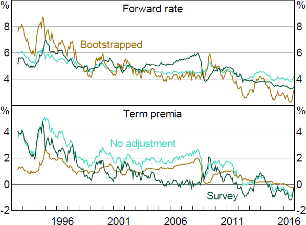
Note: Nominal ATSM with four factors.
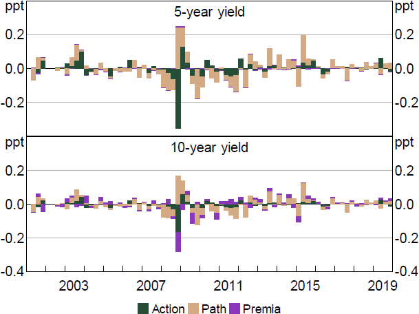
Notes: Decomposition based on regression of yield changes on shocks. Residuals excluded. Quarterly sum.
Appendix B: Additional Results
| Baseline sample | Orthogonalised | No GFC | Bootstrapped | |
|---|---|---|---|---|
| Action shock(a) | 9.84 | 6.62 | 7.68 | 8.89 |
| Path shock(b) | 0.14 | 0.34 | 0.32 | 1.31 |
| Premia shock(b) | 1.46 | 1.73 | 0.08 | 2.05 |
| 3-month OIS change(a) | 9.21 | na | na | na |
| 24-month yield change(a) | 8.32 | na | na | na |
| Action shock – quarterly(a) | 15.37 | na | 3.96 | na |
| Path shock – quarterly(b) | 1.77 | na | 0.47 | na |
| Premia shock – quarterly(b) | 2.12 | na | 0.56 | na |
| Action shock – all events(a) | 13.32 | na | na | 14.03 |
| Path shock – all events(b) | 0.90 | na | na | 1.01 |
| Premia shock – all events(b) | 1.82 | na | na | 7.01 |
|
Notes: (a) Instrumenting for first principal component of yield curve. (b) Instrumenting for second principal component of yield curve. |
||||
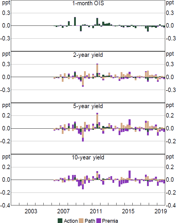
Notes: Decomposition based on regression of yield changes on shock. Residuals excluded. Quarterly sum.
Note: Dashed lines denote 90 per confidence intervals (bootstrapped).
Notes: Dashed lines denote 90 per cent confidence intervals. 10-year yield and cash rate bands excluded as their responses are constructed based on factor responses.
References
Adrian T, RK Crump and E Moench (2013), ‘Pricing the Term Structure with Linear Regressions’, Journal of Financial Economics, 110(1), pp 110–138.
Andreasen MM and A Meldrum (2013), ‘Dynamic Term Structure Models: The Best Way to Enforce the Zero Lower Bound?’, Paper presented at the Federal Reserve Bank of San Francisco Conference ‘Term Structure Modeling at the Zero Lower Bound’, San Francisco, 11 October.
Bauer MD, GD Rudebusch and JC Wu (2012), ‘Correcting Estimation Bias in Dynamic Term Structure Models’, Journal of Business & Economic Statistics, 30(3), pp 454–467.
Bauer MD and ET Swanson (2021), ‘An Alternative Explanation for the “Fed Information Effect”’, Federal Reserve Bank of San Francisco Working Paper No 2020-06.
Bauer MD and ET Swanson (2022), ‘A Reassessment of Monetary Policy Surprises and High-Frequency Identification’, NBER Working Paper No 29939.
Beckers B (2020), ‘Credit Spreads, Monetary Policy and the Price Puzzle’, RBA Research Discussion Paper No 2020-01.
Beechey M and P Österholm (2008), ‘A Bayesian Vector Autoregressive Model with Informative Steady-State Priors for the Australian Economy’, Economic Record, 84(267), pp 449–465.
Berkelmans L (2005), ‘Credit and Monetary Policy: An Australian SVAR’, RBA Research Discussion Paper No 2005-06.
Bikbov R and M Chernov (2011), ‘Yield Curve and Volatility: Lessons from Eurodollar Futures and Options’, Journal of Financial Econometrics, 9(1), pp 66–105.
Bishop J and P Tulip (2017), ‘Anticipatory Monetary Policy and the “Price Puzzle”’, RBA Research Discussion Paper No 2017-02.
Busetto F, M Chavaz, M Froemel, M Joyce, I Kaminska and J Worlidge (2022), ‘QE at the Bank of England: A Perspective on its Functioning and Effectiveness’, Bank of England Quarterly Bulletin, 2022 Q1.
Caldara D and E Herbst (2019), ‘Monetary Policy, Real Activity, and Credit Spreads: Evidence from Bayesian Proxy SVARs’, American Economic Journal: Macroeconomics, 11(1), pp 157–192.
D'Amico S and TB King (2013), ‘Flow and Stock Effects of Large-Scale Treasury Purchases: Evidence on the Importance of Local Supply’, Journal of Financial Economics, 108(2), pp 425–448.
Doko Tchatoka F and Q Haque (2021), ‘Revisiting the Macroeconomic Effects of Monetary Policy Shocks’, Australian National University Crawford School of Public Policy, Centre for Applied Macroeconomic Analysis, CAMA Working Paper 61/2021.
Duffee GR (2002), ‘Term Premia and Interest Rate Forecasts in Affine Models’, The Journal of Finance, 57(1), pp 405–443.
Finlay R and D Olivan (2012), ‘Extracting Information from Financial Market Instruments’, RBA Bulletin, March, pp 45–54.
Finlay R, D Titkov and M Xiang (2022), ‘The Yield and Market Function Effects of the Reserve Bank of Australia's Bond Purchases’, RBA Research Discussion Paper No 2022-02.
Gambetti L (2021), ‘Shocks, Information, and Structural VARs’, Oxford Research Encyclopaedia of Economics and Finance, accessed 21 November 2022. Available at <https://doi.org/10.1093/acrefore/9780190625979.013.621>.
Gertler M and P Karadi (2015), ‘Monetary Policy Surprises, Credit Costs, and Economic Activity’, American Economic Journal: Macroeconomics, 7(1), pp 44–76.
Guimarães R (2016), ‘Fool's Errand? Robust Identification of Risk Premia and Expectations in Asset Prices’, Unpublished manuscript, Bank of England, May. Previously released as Bank of England Working Paper No 489. Available at SSRN at <https://ssrn.com/abstract=2420379>.
Gürkaynak RS, B Sack and E Swanson (2005a), ‘Do Actions Speak Louder Than Words? The Response of Asset Prices to Monetary Policy Actions and Statements’, International Journal of Central Banking, 1(1), pp 55–93.
Gürkaynak RS, B Sack and E Swanson (2005b), ‘The Sensitivity of Long-Term Interest Rates to Economic News: Evidence and Implications for Macroeconomic Models’, The American Economic Review, 95(1), pp 425–436.
Hambur J and R Finlay (2018), ‘Affine Endeavour: Estimating a Joint Model of the Nominal and Real Term Structures of Interest Rates in Australia’, RBA Research Discussion Paper No 2018-02.
Hartigan L and J Morley (2020), ‘A Factor Model Analysis of the Australian Economy and the Effects of Inflation Targeting’, Economic Record, 96(314), pp 271–293.
He C (2021), ‘Monetary Policy, Equity Markets and the Information Effect’, RBA Research Discussion Paper No 2021-04.
Jääskelä J and D Jennings (2010), ‘Monetary Policy and the Exchange Rate: Evaluation of VAR Models’, RBA Research Discussion Paper No 2010-07.
Jääskelä J and P Smith (2011), ‘Terms of Trade Shocks: What are They and What Do They Do?’, RBA Research Discussion Paper No 2011-05.
Jarociński M and P Karadi (2020), ‘Deconstructing Monetary Policy Surprises—The Role of Information Shocks’, American Economic Journal: Macroeconomics, 12(2), pp 1–43.
Jentsch C and KG Lunsford (2019), ‘The Dynamic Effects of Personal and Corporate Income Tax Changes in the United States: Comment’, The American Economic Review, 109(7), pp 2655–2678.
Joslin S, KJ Singleton and H Zhu (2011), ‘A New Perspective on Gaussian Dynamic Term Structure Models’, The Review of Financial Studies, 24(3), pp 926–970.
Jurado K, SC Ludvigson and S Ng (2015), ‘Measuring Uncertainty’, The American Economic Review, 105(3), pp 1177-1216.
Kaminska I and H Mumtaz (2022), ‘Monetary Policy Transmission during QE Times: Role of Expectations and Term Premia Channels’, Bank of England Staff Working Paper No 978.
Kaminska I, H Mumtaz and R Šustek (2021), ‘Monetary Policy Surprises and Their Transmission through Term Premia and Expected Interest Rates’, Journal of Monetary Economics, 124, pp 48-65.
Kim DH and A Orphanides (2012), ‘Term Structure Estimation with Survey Data on Interest Rate Forecasts’, Journal of Financial and Quantitative Analysis, 47(1), pp 241-272.
Kuttner KN (2001), ‘Monetary Policy Surprises and Interest Rates: Evidence from the Fed Funds Futures Market’, Journal of Monetary Economics, 47(3), pp 523-544.
Lawson J and D Rees (2008), ‘A Sectoral Model of the Australian Economy’, RBA Research Discussion Paper No 2008-01.
Lucca DO and JH Wright (2022), ‘The Narrow Channel of Quantitative Easing: Evidence from YCC Down Under’, Federal Reserve Bank of New York Staff Report No 1013.
Malik S and A Meldrum (2016), ‘Evaluating the Robustness of UK Term Structure Decompositions Using Linear Regression Methods’, Journal of Banking & Finance, 67, pp 85-102.
Mertens K and MO Ravn (2013), ‘The Dynamic Effects of Personal and Corporate Income Tax Changes in the United States’, The American Economic Review, 103(4), pp 1212-1247.
Miranda-Agrippino S and G Ricco (2021), ‘The Transmission of Monetary Policy Shocks’, American Economic Journal: Macroeconomics, 13(3), pp 74-107.
Montiel Olea JL, JH Stock and MW Watson (2021), ‘Inference in Structural Vector Autoregressions Identified with an External Instrument’, Journal of Econometrics, 225(1), pp 74-87.
Nakamura E and J Steinsson (2018), ‘High-Frequency Identification of Monetary Non-Neutrality: The Information Effect’, The Quarterly Journal of Economics, 133(3), pp 1283-1330.
Nicholls DF and AL Pope (1988), ‘Bias in the Estimation of Multivariate Autoregressions’, Australian & New Zealand Journal of Statistics, 30A(1), pp 296-309.
Ramey VA (2016), ‘Macroeconomic Shocks and Their Propagation’, in JB Taylor and H Uhlig (eds), Handbook of Macroeconomics: Volume 2A, Handbooks in Economics, Elsevier, Amsterdam, pp 71-162.
Read M (2022), ‘Estimating the Effects of Monetary Policy in Australia Using Sign-Restricted Structural Vector Autoregressions’, RBA Research Discussion Paper No 2022-09.
Romer CD and DH Romer (2004), ‘A New Measure of Monetary Shocks: Derivation and Implications’, The American Economic Review, 94(4), pp 1055-1084.
Staiger D and JH Stock (1997), ‘Instrumental Variables Regression with Weak Instruments’, Econometrica, 65(3), pp 557-586.
Stock JH (2008), ‘Recent Developments in Structural VAR Modeling’, What's New in Econometrics: Time Series, Lecture 7, NBER Summer Institute, 15 July. Available at <https://www2.nber.org/WNE/slides7-14-08/Lecture7.pdf>.
Stock JH and MW Watson (2012), ‘Disentangling the Channels of the 2007–09 Recession’, Brookings Papers on Economic Activity, Spring, pp 81–135.
Stock JH and MW Watson (2018), ‘Identification and Estimation of Dynamic Causal Effects in Macroeconomics Using External Instruments’, The Economic Journal, 128(610), pp 917–948.
Copyright and Disclaimer Notice
RP Data Pty Ltd trading as CoreLogic Asia Pacific Disclaimer Notice
This publication contains data, analytics, statistics, results and other information licensed to the Reserve Bank of Australia by RP Data Pty Ltd trading as CoreLogic Asia Pacific (CoreLogic Data).
© Copyright 2023. RP Data Pty Ltd trading as CoreLogic Asia Pacific (CoreLogic) and its licensors are the sole and exclusive owners of all rights, title and interest (including intellectual property rights) subsisting in the CoreLogic Data reproduced in this publication. All rights reserved.
The CoreLogic Data provided in this publication is of a general nature and should not be construed as specific advice or relied upon in lieu of appropriate professional advice.
While CoreLogic uses commercially reasonable efforts to ensure the CoreLogic Data is current, CoreLogic does not warrant the accuracy, currency or completeness of the CoreLogic Data and to the full extent permitted by law excludes all loss or damage howsoever arising (including through negligence) in connection with the CoreLogic Data.
Acknowledgements
Thanks to Meredith Beechey-Österholm, James Morley, Matthew Read, Chris Gibbs, Bonsoo Koo, Wenying Yao and seminar participants at the RBA for their helpful comments. Thanks to Brian Tran for his measures of monetary policy uncertainty, Luke Hartigan for the measure of macroeconomic factors, Calvin He for his earlier work pulling together high-frequency yield data and Jeremy Lwin for providing updates. The views expressed in this paper are those of the authors and do not necessarily reflect the views of the Reserve Bank of Australia. The authors are responsible for any errors.
Footnotes
Economic Research Department, Reserve Bank of Australia [*]
University of Adelaide [**]
Doko Tchatoka and Haque (2021) point out that the real effects of US monetary policy shocks identified using Gertler and Karadi's (2015) approach are sensitive to the sample period. They find that once the Volcker disinflation period is left out and one focuses on the post-mid-1980s period, policy shocks have no significant effects on output, despite large movements in credit costs. [1]
We only use data up to 2016 to estimate the parameters to avoid any possibility of the proximity of the effective lower bound affecting the estimates. See Appendix A for further discussion. [2]
We use two factors following KMS, though there is evidence that one factor may be sufficient to encapsulate changes in expected rates. The first factor accounts for around 98 per cent of variation, while the second accounts for around 2 per cent and others near zero. This finding is similar when using forward rates as well as expected average rates. [3]
Including the other events doesn't change the factor loadings substantially. However, if we focus only on other events the loadings on the Action and Path shocks have a stronger downward and upward slope, respectively (Figure B1). [4]
While the shocks look potentially autocorrelated, there is no significant evidence of autocorrelation for the Action and Premia shocks. In the sample, the Path shocks do appear moderately positively autocorrelated. While this is somewhat surprising, it is broadly consistent with evidence that participants have learnt about the RBA's reaction function over time, as discussed below. Once the component that is predictable based on other available economic information is removed, the autocorrelation is no longer evident. [5]
These shares are averages across the entire yield curve. Action shocks tend to play a relatively more important role at the shorter end of the curve, while Path and Premia shocks play a more important role further out. [6]
If we fail to enforce the same loading, the loadings change substantially. Moreover, the second raw factor accounts for a substantially larger share of variation in yields – around 15 per cent. This provides more evidence that announcement days contain much more information than other days. [7]
Despite the different loadings for the shocks, these shares are similar if we estimate the model only on other events. [8]
References to such risks remained high going forward, suggesting potential change in communication strategy. [9]
More precisely, this is the conditional volatility of the residual from a forecasting model of the 3-month OIS, similar in spirit to Jurado, Ludvigson and Ng (2015). [10]
We use the final, rather than the original, vintage of the data. However, given many of the variables are not revised (i.e. financial market variables) this is unlikely to be a major issue. Moreover, unless the RBA could predict the data revisions, both the RBA and market participants had the same information set, so we are simply introducing noise into our RHS variables. Nevertheless, we make sure the data release was available at the time of the policy meeting. [11]
As in KMS we do not account for the fact that the shock is a generated regressor, given the difficulty in bootstrapping to include the ATSM step. We also implement the wild bootstrap as in Gertler and Karadi (2015). However, Jentsch and Lundsford (2019) show that the wild bootstrap is generally not asymptotically valid for inference about impulse response functions in IV-SVARs and propose a block bootstrap instead. To ensure that our results are not driven by the wild bootstrap procedure we conduct robustness checks using Bayesian local projection and find similar results regarding significance (Figure B8). [12]
The results are also broadly consistent if we orthogonalise the shocks with respect to recent economic outcomes, or use an ATSM with a bootstrap adjustment instead of surveys as in KMS (see Figure B3). [13]
Taking the point estimates at face value we see some evidence that the shocks are picking up signalling about future economic outcomes, consistent with the results in KMS. The shocks are associated with an immediate increase in longer-term interest rates, but a future increase in the cash rate. Conditions initially improve, with housing prices rising alongside dwelling approvals and retail sales, with these effects tending to wane over time. Nevertheless, given the weak instruments issue these results shouldn't be given much credence. [14]
Finlay et al (2022) mainly focus on open-to-close changes. For simplicity we focus on previous close-to-close changes. [15]
The relatively restrictive error assumption used here, and throughout the paper, is unlikely to hold in the data. While we could allow for more complex error structures, doing so would significant increase the complexity of the model. Moreover, Bikbov and Mueller (2011) find that doing so helps models match higher-order moments of the data, but not the first moments (i.e. yields). [16]