RDP 2023-04: Can We Use High-frequency Yield Data to Better Understand the Effects of Monetary Policy and Its Communication? Yes and No! 3. Documenting Shock Measures Pre-COVID-19
May 2023
- Download the Paper 1.43MB
As discussed above, KMS suggest a new approach to identifying monetary policy shocks using high-frequency data that is able to separate out the effects of action, signalling/forward guidance, and effect on term premia. Specifically, KMS suggest a three-step approach to constructing more interpretable monetary policy shocks:
- Gather high-frequency measures of surprise yield changes.
- Decompose changes in yields into changes in expected policy rates and changes in premia.
- ‘Reshape’ these changes in expected rates and premia to capture shocks to the current policy rate, to the expected future path of policy rates, and to premia or uncertainty.
3.1 Gathering high-frequency yield changes
As noted above, the KMS approach builds off the high-frequency identification literature, taking changes in yields over tight windows around events as exogenous monetary policy shocks. For this, we use data on overnight indexed swaps (OIS) at fixed maturities of 1 week, 1 to 6 months, 9 months, and 12 months, as well as yields on all outstanding nominal Australian Government securities with at least 1 year to maturity. These are measured in a reasonably tight window of 30 minutes before the relevant event, and 90 minutes after. We use these data to fit a zero-coupon yield curve just before and after the announcement, following the approach of Finlay and Olivan (2012).
Our main focus is on monetary policy announcements, which is consistent with much of the literature. We collect data on meetings covering the period from 2002 to 2019.
We also consider the broader set of events examined in He (2021), though we only incorporate data from 2006 to 2019 (as earlier data were not available). This includes speeches, release of the Board minutes, and release of the Statement on Monetary Policy. Considering these extra events not only broadens our information set in general, but may also be particularly useful in identifying shocks to the path of expected interest rates if these longer-form releases provide a more detailed assessment of the likely path for interest rates.
Table 1 provides some statistics on these changes. Variation in yields tends to be higher on monetary policy announcement days, particularly for shorter maturities, with much of the variation occurring during the tight event window. On average across the sample, other event days look fairly similar to the full sample, with the events themselves being associated with relatively minimal variation in yields. This is consistent with the findings in He (2021), though as he notes and we discuss below, some have had larger effects, particularly around the GFC.
| 1-year | 3-year | 5-year | 10-year | Observations | |
|---|---|---|---|---|---|
| Daily change | |||||
| Full sample | 0.033 | 0.043 | 0.044 | 0.046 | 3,714 |
| Monetary policy announcement day | 0.050 | 0.051 | 0.051 | 0.047 | 199 |
| Other event day | 0.029 | 0.042 | 0.042 | 0.042 | 523 |
| Change during window around announcements | |||||
| Monetary policy announcement window | 0.035 | 0.039 | 0.031 | 0.023 | 199 |
| Other event window | 0.013 | 0.018 | 0.015 | 0.015 | 523 |
| Sources: Authors' calculations; RBA; Refinitiv; Yieldbroker | |||||
3.2 Decomposing yield curve changes into changes in expected rates and premia
Following KMS, we decompose changes in the yield curve into changes in the expected path of interest rates and changes in premia by employing a standard ATSM, which is designed to model the future path of interest rates and premia based on data on yields. Our ATSM differs slightly from KMS (for details see Appendix A). First, we use a slightly different estimation procedure, suggested by Adrian, Crump and Moench (2013). But more importantly, we incorporate surveys into the model to avoid small sample biases, similar to Kim and Orphanides (2012) and Guimarães (2016), rather than using statistical techniques as in KMS. As discussed in Appendix A, this leads to a more plausible path for expected interest rates and term premia. It also affects what the model assigns as Path and Premia shocks, affecting our estimates of the effects of these shocks.
Having estimated the model parameters, we can then apply the ATSM to look at the estimated path of interest rates and term premia, before and after monetary policy announcements or other events.[2] For example, Figures 1 and 2 show the yields, expected policy rates and premia just before and after the May 2016 monetary policy announcement where a 25 basis point cut in the cash rate to 1.75 per cent was announced. Yields fell after the announcement with much of the decline reflecting lower current and expected policy rates. Premia also declined, potentially suggesting some decline in uncertainty about future rates.
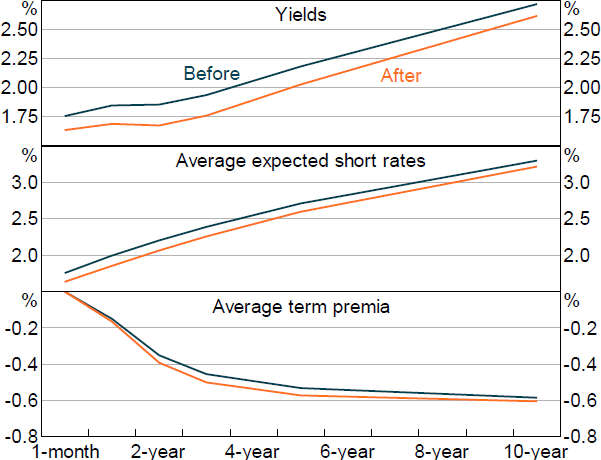
Note: Before is 30 minutes before monetary policy announcement, after is 90 minutes after monetary policy announcement.
Sources: Authors' calculations; Refinitiv; Yieldbroker
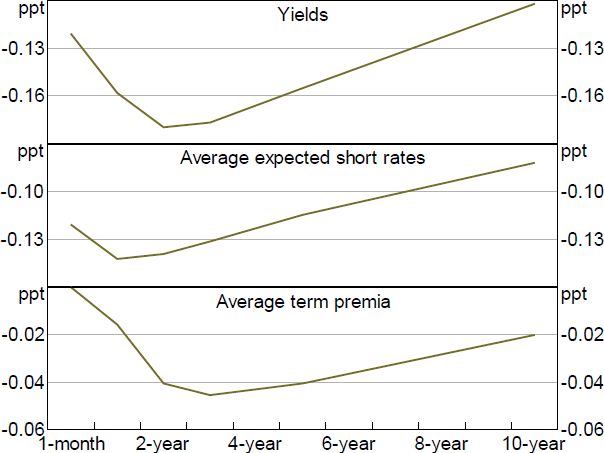
Sources: Authors' calculations; Refinitiv; Yieldbroker
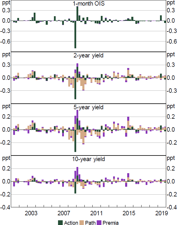
Figure 3 summarises these changes over time at a few points on the yield curve. For monetary policy announcements, changes in expected policy rates tend to be the most important aspect of yield changes, even at longer horizons. But changes in term premia can be quite important as well. For example, premia spiked around policy announcements during the GFC in late 2008, offsetting some of the effects that lower rate expectations had in lowering longer-term yields. Focusing on other events, the figure also shows that while the average effect of these events is smaller, during certain periods these events have had sizable effects on yields, indicating that they can potentially provide useful extra information on monetary policy shocks.
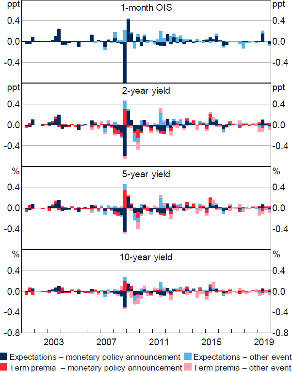
Note: Quarterly sum.
It is interesting to compare these results to an average day in the sample, as this can provide a sense of whether expected rates play a relatively larger role on monetary policy event days. To consider this, we run the ATSM over daily changes in yields across all days in the sample period (from 2002 to 2019). Perhaps unsurprisingly, on days with monetary policy announcements a far larger share of variation in yields reflects changes in expected interest rates compared with an average day (Table 2).
When we focus on non-policy announcements (e.g. speeches), changes in expected rates also play a larger role than premia in driving variation in yields, though typically not to the same extent as around monetary policy announcements. So while these other events primarily contain information about future interest rates, the composition of information released during these events is more skewed towards uncertainty or risk around the path of rates than in monetary policy announcements.
| 1-year | 3-year | 5-year | 10-year | |
|---|---|---|---|---|
| Daily change | ||||
| Full sample | 58 | 47 | 35 | 14 |
| Monetary policy announcement day | 72 | 59 | 50 | 25 |
| Other event day | 64 | 51 | 49 | 30 |
| Change during window around announcement | ||||
| Monetary policy announcement window | 95 | 79 | 75 | 58 |
| Other event window | 72 | 49 | 49 | 31 |
|
Sources: Authors' calculations; RBA; Refinitiv; Yieldbroker |
||||
3.3 Decomposing yield curve changes into changes in Action, Path and Premia shocks
While the above decomposition provides some useful extra information, it still doesn't fully differentiate between the different facets of monetary policy. For example, in the May 2016 announcement did the fall in the average expected policy rate over the next two years reflect the cut in the cash rate, or did it reflect forward guidance or signalling about the state of the economy and rates in the future? Equally, how much of the change in premia is directly related to changes in expected interest rates, which could, in turn, affect investors' views of economic conditions and therefore required term premia, and how much reflected reduced uncertainty about the future as a result of the central bank's communications?
To better understand these different facets of policy, KMS suggest adjusting the above decomposition to capture three distinct and more interpretable shocks:
- Action shocks: changes in expected policy rates flowing from changes in the current policy rate.
- Path shocks: changes in the expected path of policy rates unrelated to changes in the current policy rate (e.g. due to forward guidance or signaling).
- Premia shocks: changes in term premia unrelated to changes in policy rate expectations.
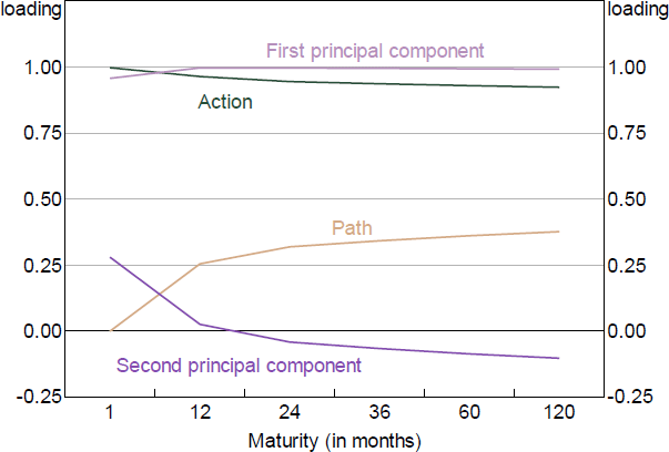
The Action and Path shocks are constructed by taking the first two principal components of changes in expected rates across the curve (i.e. ‘factors’), which summarise the changes, and transforming them so they have a cleaner interpretation. We rotate the factors such that one has no loading on the short-term interest rate: the Path shock. The other is allowed to load on the short rate: the Action shock. This is similar to the approach taken by Gürkaynak et al (2005a), but they apply it to the raw yield curve rather than first removing term premia.[3]
Focusing on policy announcement days, the factor loadings end up looking similar to a ‘level’ and ‘slope’ factor, which is a common finding when taking principal components of a yield curve (e.g. Hambur and Finlay (2018); Figure 4).[4] Action shocks lead to a fairly consistent increase in expected rates across the curve. Path shocks by construction have no effect on current rates, but larger effects on future interest rates, so lead to a steeper yield curve (all else equal).
To construct the Premia shock we compute the residual from a regression of the term premia changes on the above factors, which removes the influence of expected rate changes. We then take the first principal component of these residuals to summarise the changes across all maturities. KMS take the additional step of rotating the term premia so that it does not load on short-term premia, similar to the adjustment made to construct the Path factor. We experimented with this approach and it does not substantially change the results, but does lower the explanatory power of the Premia shocks.
Figure 5 shows the contribution of these different facets of monetary policy shocks to yields over time, focusing on monetary policy announcements. Much of the variation in yields across the curve reflects current policy actions (~65 per cent), and these shocks show a reasonable correlation with the measures proposed in Beckers (2020): around 0.5.[5] Changes in the expected path also play an important role (~20 per cent), while changes in uncertainty/premia account for only a small share (~10 per cent).[6]
Notes: Decomposition based on regression of yield changes on shocks. Residuals excluded. Quarterly sum.
Similar to the above findings, the dominance of the Action shock seems to be particularly evident on monetary policy announcement days. If we run the model over all days from 2002 to 2019 (and enforce the same factor loadings), the Path shock accounts for around 1.5 times as much variation in yields as the Action shock across different maturities.[7] In contrast, on announcement days the two play a broadly similar role (and the Action shock is more important within the window). Similarly, focusing on other event days the Action shock accounts for only around 15 per cent of variation, compared with 60 per cent for the Path and 20 per cent for the Premia shock.[8] This suggests that monetary policy announcements are unique in containing mainly information related to interest rates in the immediate future (perhaps unsurprisingly).
Even if Path and Premia shocks are relatively less important overall in policy announcement events, they have played crucial roles at different stages, particularly for medium-to-longer-term yields. For example, Path shocks consistently lowered medium-term yields during the early stages of the GFC in early and mid-2008. To understand this, we use simple text analysis of the policy announcement. We find that the negative path shocks coincided with increased references to softening credit and economic conditions, volatile overseas outcomes, and economic risks, as evident from the increase in the number of references to risk in the monetary policy announcements (Figure 6).[9]
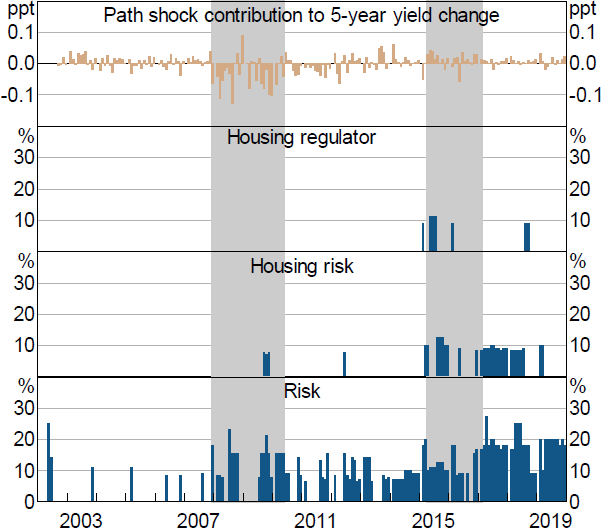
Notes: Housing words include: dwelling prices, housing credit, housing market, housing conditions and household debt. Risk words include: downside risk, concern(s) and risk(s). Regulator words include: regulator(s) and APRA. Abating words include: eased, declining, decline(s), easing, fall(s) and abate. Housing regulator includes a housing word and a regulator word. Housing risk includes a housing word and a risk word. All groups exclude any abating words.
Sources: Authors' calculations; RBA
Similarly, Path shocks seem to have consistently raised short- to medium-term yields during the mid-2010s. This was also evident for other events (see Figure B2). One potential explanation could be that increased references to housing prices and risks caused markets to adjust their expectations for future policy rates higher. To consider this, we again use simple text analysis to look for references to risks in housing markets or to the regulator (with no offsetting word) in monetary policy announcements. As shown in Figure 6, references to these risks have tended to coincide with positive path shocks. While this finding is by no means causal and conclusive, it does provide some evidence that the shocks are able to parse some of the relevant information being communicated about the future path of interest rates.
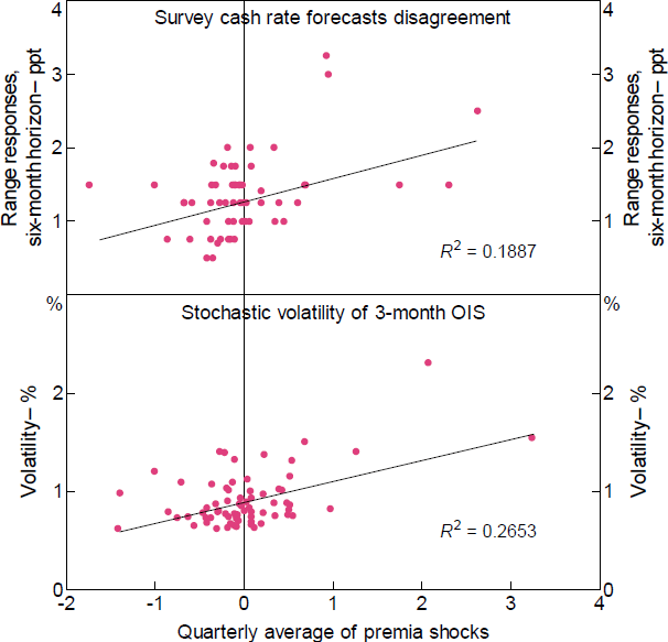
Meanwhile Premia shocks appear to be related to monetary policy uncertainty. There were large Premia shocks around monetary policy announcements during the GFC, a period of heightened uncertainty. Moreover, there is a reasonable positive correlation between various proxies for monetary policy uncertainty and Premia shocks. For example, forecaster disagreement regarding the future cash rate as measured in the RBA Survey of Market Economists, a proxy for uncertainty, has a moderate correlation with the size of the Premia shocks in that quarter (Figure 7, top panel). This relationship is not present when looking at the Action or Path shocks, and does not simply reflect the GFC period. Similarly, there is a moderate correlation between the (conditional) volatility of the 3-month OIS and the Premia shock in a given month.[10]
Sources: Authors' calculations; RBA
Finally, one natural question about these shocks is whether they are truly exogenous and unpredictable. Several papers have argued that high-frequency shocks can still be endogenous if the central bank has some additional economic information that it communicates, or if market participants misunderstand the central bank's responses to data (Nakamura and Steinsson 2018; Bauer and Swanson 2021, 2022). The former will naturally be captured in the Path shocks as this additional information about future outcomes should influence expected future interest rates. Separating this out, and being able to look at this aspect versus the effect of current actions is a key benefit of the KMS approach. The latter remains a cause for concern and so we explore it below.
To understand whether market participants systematically misinterpret the RBA's response to incoming data, we consider whether they could have ‘predicted’ the shocks using available data. Specifically, we regress each shock on various measures of economic and credit conditions which include the following: changes in the unemployment rate and (log) employment over the preceding twelve months, and three-month changes in the (log) TWI, money market spread (3-month BBSW less OIS), the US commercial paper spread, the second principal component of the yield curve (strongly related to its slope), (log) commodity prices, (log) ASX 200, the US VIX and the US corporate bond spread (BAA). These variables are motivated by Bauer and Swanson (2021, 2022) and Beckers (2020). The regression is run separately while including and excluding the GFC period, to allow for the fact that the relationships may have changed during this period.[11]
We find that these factors explain around 20 per cent of the variation in Action shocks, 25 per cent of the variation in Path shocks and 15 per cent of the variation in Premia shocks when the GFC is included in the sample. If we exclude the GFC, the share for the Action shocks declines substantially but remains the same for the other two components. This suggests that while the Action shocks are truly unpredictable, with the benefit of hindsight, market participants may have been able to predict the other shocks. It also suggests that the nature of what is being identified as a shock during the GFC could differ from the rest of the sample, potentially reflecting less efficient price discovery and incorporation of information during this volatile period.
How can we explain this predictability and the apparent systematic misunderstanding of the RBA's reaction function, at least with respect to the future stance of policy? One explanation is that markets learn about the reaction function over time (Bauer and Swanson 2021, 2022). Relatedly, the reaction function could change over time, and agents may be slow to learn about those changes. This could explain the autocorrelation observed in the Path shocks, which is removed once we orthogonalise the shocks with respect to available data. In either case, the results speak to the importance of effectively communicating the RBA's reaction function.
Interestingly, if we focus on the other events alone, the degree of predictability is far lower, in the region of 5 to 10 per cent. This suggests that these events contain relatively more exogenous information.
In terms of using these shocks as instruments for monetary policy, the predictability of the Path and Premia shocks indicates that they are unlikely to be a valid instrument as they may be correlated with other structural shocks or expected future economic outcomes. That said, the direction of the bias will be less clear, and will be dependent on whether participants over or underweight certain variables. Rather than exploring deeply the nature of the systematic error, we simply consider the macroeconomic effects of the shocks with and without the orthogonalisation step in the next section.
Footnotes
We only use data up to 2016 to estimate the parameters to avoid any possibility of the proximity of the effective lower bound affecting the estimates. See Appendix A for further discussion. [2]
We use two factors following KMS, though there is evidence that one factor may be sufficient to encapsulate changes in expected rates. The first factor accounts for around 98 per cent of variation, while the second accounts for around 2 per cent and others near zero. This finding is similar when using forward rates as well as expected average rates. [3]
Including the other events doesn't change the factor loadings substantially. However, if we focus only on other events the loadings on the Action and Path shocks have a stronger downward and upward slope, respectively (Figure B1). [4]
While the shocks look potentially autocorrelated, there is no significant evidence of autocorrelation for the Action and Premia shocks. In the sample, the Path shocks do appear moderately positively autocorrelated. While this is somewhat surprising, it is broadly consistent with evidence that participants have learnt about the RBA's reaction function over time, as discussed below. Once the component that is predictable based on other available economic information is removed, the autocorrelation is no longer evident. [5]
These shares are averages across the entire yield curve. Action shocks tend to play a relatively more important role at the shorter end of the curve, while Path and Premia shocks play a more important role further out. [6]
If we fail to enforce the same loading, the loadings change substantially. Moreover, the second raw factor accounts for a substantially larger share of variation in yields – around 15 per cent. This provides more evidence that announcement days contain much more information than other days. [7]
Despite the different loadings for the shocks, these shares are similar if we estimate the model only on other events. [8]
References to such risks remained high going forward, suggesting potential change in communication strategy. [9]
More precisely, this is the conditional volatility of the residual from a forecasting model of the 3-month OIS, similar in spirit to Jurado, Ludvigson and Ng (2015). [10]
We use the final, rather than the original, vintage of the data. However, given many of the variables are not revised (i.e. financial market variables) this is unlikely to be a major issue. Moreover, unless the RBA could predict the data revisions, both the RBA and market participants had the same information set, so we are simply introducing noise into our RHS variables. Nevertheless, we make sure the data release was available at the time of the policy meeting. [11]