RDP 2023-04: Can We Use High-frequency Yield Data to Better Understand the Effects of Monetary Policy and Its Communication? Yes and No! 4. The Effects of Monetary Policy Shocks
May 2023
- Download the Paper 1.43MB
The above section highlights that these new measures of monetary policy shocks contain relevant information about monetary policy and its communication. Given they seem to capture different facets of monetary policy, they may have different macroeconomic effects, and therefore this decomposition could potentially provide useful quantitative estimates of how monetary policy and its communication affect the macroeconomy.
To consider this we use an instrumental-variable structural vector autoregression (IV-SVAR) approach. This approach was pioneered by Stock (2008), Stock and Watson (2012, 2018) and Mertens and Ravn (2013). The idea behind this approach is to use instruments (in our case policy surprises as discussed above) to identify (different facets of) monetary policy shocks from a reduced form VAR.
More precisely, we consider the following proxy SVAR model (see also Doko Tchatoka and Haque (2021))
where Yt is an n×1 vector of endogenous variables, ut is an n×1 vector of reduced-form innovations, p is the number of lags, and are n×n matrices of unknown coefficients. The reduced-form innovations are related to the structural shocks as follows:
where A0 is an n×n non-singular matrix and the structural shocks are assumed to be serially and mutually uncorrelated and satisfy the following:
The variance-covariance matrix of the reduced-form innovations is given by
Yt has a structural moving average (MA) representation
where B = (B1, B2,...,Bp) and Ck (B) highlight the dependence of the MA coefficients on the autoregressive coefficients in B, that is
with C0(B) = In and Bm = 0 for m > p (e.g. Montiel Olea, Stock and Watson 2021).
The structural impulse response function is the response of Yi,t+k to a one-unit change in , which is given by
where ei and ej denote the ith and jth columns of the identity matrix In, respectively.
Following Gertler and Karadi (2015), we identify the policy shock using an external instrument. Let zt denote an external instrument and be an (n–1)×1 vector of structural shocks other than the monetary policy shock. The key identification assumption in the external instrument approach is that zt is correlated with but uncorrelated with . Stock and Watson (2018) and Montiel Olea et al (2021) show that if this identifying assumption holds, then one can identify the structural shock of interest.
Our baseline VAR is estimated (using ordinary least squares) at a monthly frequency. The variables included in the IV-SVAR are: unemployment rate, (log) retail sales, (log) housing prices, (log) dwelling approvals, the mortgage spread (variable owner-occupier rate less cash rate; adjusted for a break around the GFC), the (log) nominal TWI, and the first two principal components of the yield curve. The VAR is estimated over the sample from January 1994 to December 2019, while the high-frequency surprises that are used to identify the structural policy shocks only begin in 2002. We examine the effect of each of the surprise components one-by-one, using them as instruments for the yield curve factors. Confidence bands are constructed using a wild bootstrap.[12]
Many papers incorporate specific interest rates, such as the cash rate, or other short-term interest rates. Given some of our shocks directly affect longer-term rates and not short-term rates, we also need to incorporate longer-term rates. Rather than choosing yields of certain maturities, we use the first two principal components of the yield curve in the VAR, similar to KMS. This allows us to flexibly account for the effect of the shocks, rather than taking a stand on the most relevant maturity, although it does make scaling and interpreting the shocks more challenging. We consider the effect of a shock that leads to a one standard deviation increase in one of the factors. We can then use the factor loadings to estimate the effect on relevant interest rates.
4.1 Monthly VAR
4.1.1 Action shocks
Figure 8 shows the impulse responses from an Action shock focusing on monetary policy announcements. The shock is scaled to lead to a one unit increase in the first principal component of the yield curve, which equates to around a 200 basis point increase in the cash rate. The shock has a robust F-statistic for instrument strength of around 10, which is the level often used to assess instrument strength (Staiger and Stock 1997; Table B1).
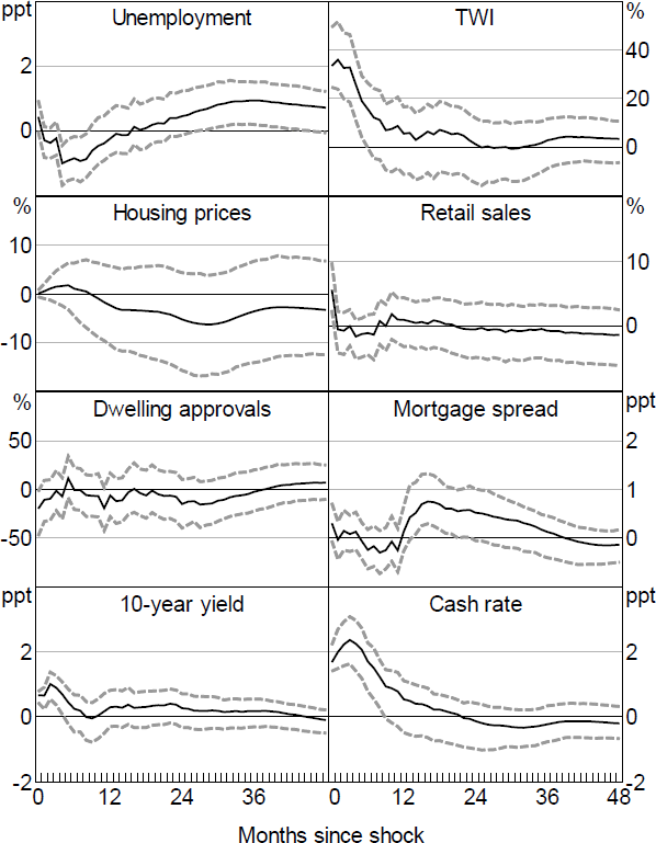
Note: Dashed lines denote 90 per cent confidence intervals (bootstrapped).
The responses are largely consistent with what would be expected from a standard contractionary monetary policy shock. Both short- and longer-term interest rates rise, the exchange rate appreciates instantaneously, and the shock leads to an eventual increase in unemployment, while housing prices decline somewhat over time.
Nevertheless, there are some surprising dynamics as unemployment initially declines. Part of this appears to reflect the inclusion of the GFC period, with the extent of the decline tending to be much smaller if this period is removed (Figure B3). Similarly, the response of the TWI is also somewhat larger than would generally be expected but becomes smaller if the GFC period is removed.
Overall, the results are very similar to those obtained from simpler approaches, such as taking information directly from the yield curve without applying an ATSM. For example, using just the change in the 3-month or 2-year OIS rate around the Board meeting leads to very similar results, as does simply taking the first factor of the change in expected short rates from the ATSM changes without rotating to extract the Action and Path shocks (Figure B6).[13] This provides some initial evidence that suggests that the identified Path and Premia shocks might have a fairly small systematic effect on economic outcomes.
Expanding the information set to include other events has relatively little effect on the results (Figure B7). This is unsurprising given the earlier findings that Action shocks were mainly relevant on policy announcement days.
4.1.2 Path shocks
The Path shock appears to be a fairly weak instrument for monetary policy shocks, with a very low F-statistic (Table B1). Accordingly, the effects are imprecisely estimated with large confidence bands and as such Figure 9 only reports the point estimates.[14] Moreover, the responses are not particularly robust to specification changes such as removing the GFC period or orthogonalising the shocks (Figure B4).
Expanding the information set to include the broader set of events does little to change the results, which remain poorly identified with a very low F-statistic (Table B1). This remains the case when we use only the non-monetary policy announcement events.
One explanation for the fact that Path shocks appear not to have significant macroeconomic effects is that policy and other announcements have little to no economic effects via signalling or information channels, unlike in the United States (per KMS). This would be somewhat consistent with He (2021) who finds little evidence of signalling effects in RBA announcements apart from speeches when looking at equity prices using a simpler approach with high-frequency yields.
Note: No responses are significant.
Another potential explanation is that Path shocks capture different aspects of the RBA's communication at different points in time. As discussed in Section 3, in the lead up to the GFC the declines in rates appear to signal downside risks to future economic conditions, consistent with standard signalling channels. But in the mid-2010s, the increases in future expected policy rates appear to reflect the RBA indicating that rates may remain elevated due to concerns over potential risks in the housing market, a pure monetary policy shock that would weigh on macroeconomic outcomes. In both cases the Path shocks would be associated with weaker economic conditions, but one set was positive and the other was negative, so the average effect of Path shocks may net out when used in the SVAR.
4.1.3 Premia shocks
As in KMS, the responses to Premia shocks are difficult to interpret and do not conform to a standard view of the impact of uncertainty (Figure 10). Moreover, the impulse responses are highly sensitive to the inclusion of the GFC period, and are imprecisely estimated, consistent with Premia shocks being a weak instrument for changes in the yield curve, with a very low F-statistic (Table B1; Figure B5).
Note: No responses are significant.
Again, expanding the information set does little to change the results. The Premia shocks still represent weak instruments, with poorly identified responses.
4.2 Quarterly VAR
As the policy shocks are constructed at a monthly frequency, we use a monthly VAR for the baseline analysis. To consider whether these shocks are able to overturn the well-known price puzzle, we also estimate a quarterly VAR. The variables are largely the same, however, we include the log trimmed mean CPI in the model and replace retail sales with log GDP and the nominal TWI with the real TWI. We sum the shocks in each quarter to get a quarterly shock series.
Figure 11 shows the results for the Action shock. Overall, the responses of most variables are similar to the monthly results. However, inflation rises following the shock, suggesting that the Action shock still contains some endogenous component. Orthogonalising the shocks does little to change this result, nor does removing the GFC period. This suggest that the high-frequency identification approach itself is unable to solve the price puzzle.
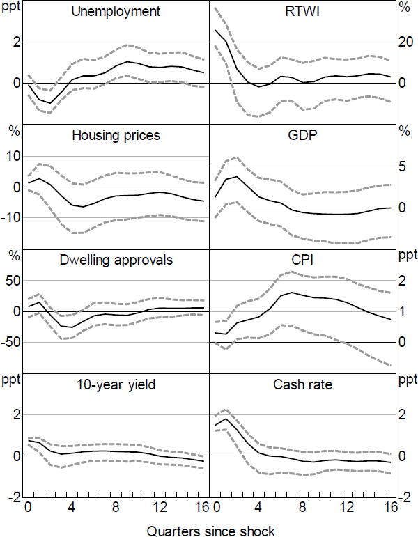
Note: Dashed lines denote 90 per cent confidence intervals (bootstrapped).
4.3 Robustness
We perform a number of checks to assess the robustness of the results for both the monthly and quarterly VAR. As we note above, we consider removing the GFC period. The main systematic difference is to the results for the Action shock, with the surprising initial decline in unemployment being less significant this time.
As noted above, we also consider orthogonalising the shocks to remove any systematic relationship with variables that were known at the time, removing what Bauer and Swansson (2022) refer to as the ‘Fed response to news’ effect. Doing so has little implication for the Action shocks but leads to much more muted responses for the Path shocks. This is consistent with the interpretation of these shocks as capturing RBA signals about future outcomes that are based on available news on recent outcomes, with markets systematically underappreciating this additional news.
In terms of the price puzzle, our results may reflect an information sufficiency issue in small-scale SVARs (e.g. Gambetti 2021). For example, Hartigan and Morley (2020) find this information deficiency to be relevant for Australia and resolve the price puzzle using recursive identification in a factor augmented VAR (FAVAR) with two factors extracted from a large macro dataset. Accordingly, we incorporate the macro factors from Hartigan and Morley to increase the information set in our estimated VAR. However, the effects of the Action shock remain largely unchanged with the price puzzle still remaining unresolved in our high-frequency identification setting.
As an alternative approach to the IV-SVAR we also consider a Bayesian local projections model, as in KMS. The results are generally quite similar to our baseline results, with the Action shock leading to an economic contraction, while the other shocks lead to poorly identified economic responses (Figure B8). This helps to address concerns around our choice of bootstrapping methods (see above).
The main other robustness check we consider is changing the ATSM. In particular, rather than incorporating surveys into the ATSM, we account for the small-sample bias using bootstrapping, similar to the statistical approach taken in KMS. Taking this approach leads to very similar estimated effects for the Action shocks (Figure B3). The main differences are evident in the Path and Premia shocks with the responses tending to be more muted (Figures B4 and B5).
Our finding that the specification of the ATSM matters for the estimation results is not surprising. As discussed in Appendix A, the choice of small-sample adjustment can lead to very different estimated paths for future expected interest rates and term premia, with the survey model providing a more sensible account of history. This suggests that in adopting the KMS approach, it is important to think about the specification of the ATSM, as it can have substantial implications for what the model interprets as Path and Premia shocks. While this doesn't seem to be important in the Australian case, given only the Action shock has macroeconomic effects, it could be more important in other countries.
Footnotes
As in KMS we do not account for the fact that the shock is a generated regressor, given the difficulty in bootstrapping to include the ATSM step. We also implement the wild bootstrap as in Gertler and Karadi (2015). However, Jentsch and Lundsford (2019) show that the wild bootstrap is generally not asymptotically valid for inference about impulse response functions in IV-SVARs and propose a block bootstrap instead. To ensure that our results are not driven by the wild bootstrap procedure we conduct robustness checks using Bayesian local projection and find similar results regarding significance (Figure B8). [12]
The results are also broadly consistent if we orthogonalise the shocks with respect to recent economic outcomes, or use an ATSM with a bootstrap adjustment instead of surveys as in KMS (see Figure B3). [13]
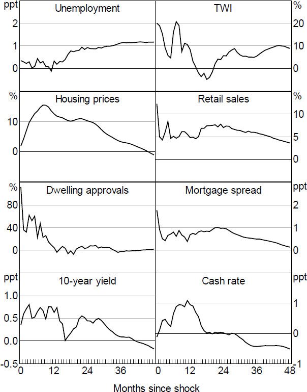
Taking the point estimates at face value we see some evidence that the shocks are picking up signalling about future economic outcomes, consistent with the results in KMS. The shocks are associated with an immediate increase in longer-term interest rates, but a future increase in the cash rate. Conditions initially improve, with housing prices rising alongside dwelling approvals and retail sales, with these effects tending to wane over time. Nevertheless, given the weak instruments issue these results shouldn't be given much credence. [14]