RDP 2021-10: The Rise in Household Liquidity 6. The Rise in Household Liquidity and Falling Interest Rates
November 2021
- Download the Paper 1.71MB
Next, we consider how the rise in household liquidity and mortgage debt is linked to the trend decline in interest rates that has been observed over recent decades in Australia and elsewhere. Identifying the effects of interest rates on the liquidity of household balance sheets is challenging. This is because lower interest rates can have both direct and indirect effects on aggregate household liquidity and mortgage debt, and these effects work in opposite directions. First, lower interest rates can contribute to higher housing prices and debt relative to incomes. This increases the value of illiquid assets on household balance sheets, particularly for home buyers that have taken on new loans. In this case, lower interest rates increase mortgage debt inflows. But lower interest rates also make it easier to repay existing debts through prepayments, thereby increasing mortgage debt outflows. The net effect on the change in the stock of mortgage debt (relative to income) depends on which effect dominates.
6.1 The effect of interest rates on aggregate liquidity and mortgage debt
We first study the effects of changes in interest rates on aggregate mortgage debt and household liquidity buffers. For this, we estimate a series of impulse response functions (IRFs) using the local projections (LP) method of Jordà (2005).[16] For each forecast horizon ( h ) we run a regression of the quarterly (cumulative) change in liquidity buffer on unexpected changes in the cash rate, or monetary policy ‘shocks’ (as measured by Beckers (2020)) ( mp ),[17] as well as controls for the lagged value of the buffer:
The impulse response of the cumulative change in liquidity buffer to the monetary policy shock is traced out by the estimates of the . For example, when h = 10, the left-hand side variable is the difference in the liquid asset-to-income ratio at quarter 10 and the liquid asset-to-income ratio at the time of the monetary policy shock (at quarter 0). The sample covers the period from 1994:Q1 to 2019:Q3 due to sample coverage of the monetary policy shock series.
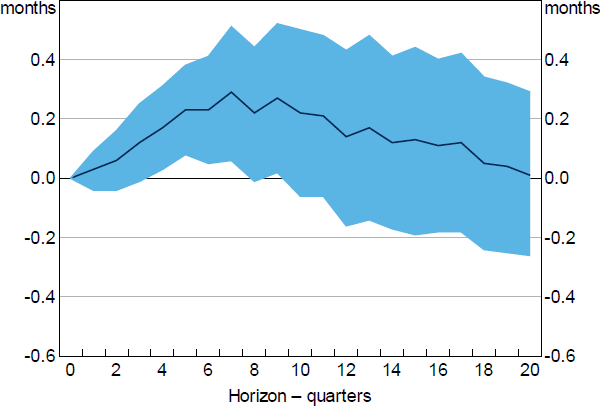
The impulse response estimates indicate that the effect of a temporary monetary policy shock on household liquidity peaks between five to eight quarters after the shock, with the effect gradually fading beyond eight quarters (Figure 17). These effects are statistically significant. However, the economic magnitude is relatively small with an unexpected 1 percentage point reduction in the cash rate being associated with aggregate liquidity buffers rising by about 0.3 months of income at the peak. We also find that this effect comes through a combination of increases in both the value of bank deposits and equities in response to temporarily lower interest rates.
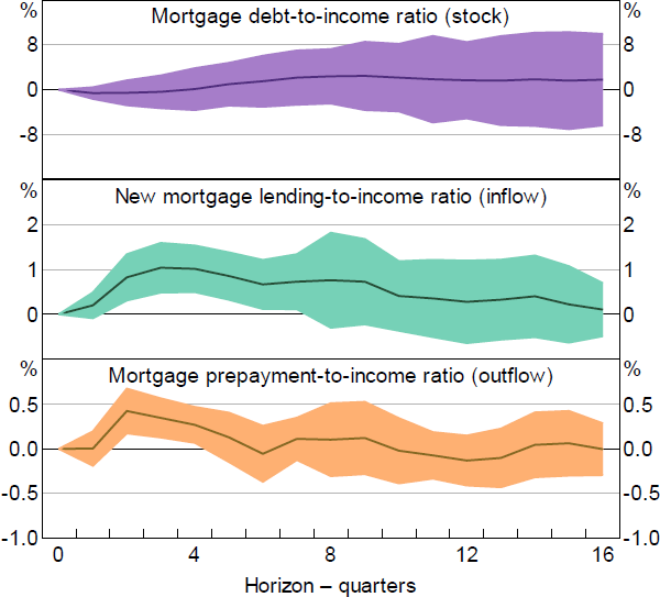
To isolate the effect of interest rates on liquidity through the housing market we repeat the same exercise and estimate IRFs for the effect of interest rate shocks on mortgage debt, including both the inflows (new loans) and outflows (prepayments). This allows us to explore the direct and indirect effects of interest rates on liquid assets through the housing market.

Note: Shaded area represents confidence interval based on +/– 2 standard errors
Sources: ABS; APRA; Authors' calculations
For this exercise, we measure mortgage inflows based on the value of new mortgage loans, excluding refinancing, each quarter as reported by the ABS. We then measure mortgage outflows as the residual difference between inflows and the change in the stock of mortgage debt. The inflows, outflows and the stock of mortgage debt are each scaled by household disposable income. The time window is restricted to the period between 2002:Q1 to 2019:Q3 as the ABS estimates of new lending begin at this time. The lack of business cycle fluctuations makes it harder to cleanly identify the effects of interest rates.[18]
An unexpected 100 basis point reduction in the cash rate is associated with an increase in new loans (relative to income) of 1 per cent after three to four quarters (Figure 18). The effect persists for about two years. This indicates that lower interest rates support new borrowing and the value of (illiquid) housing assets. But lower interest rates are also associated with a higher share of income going to prepayments. An unexpected 100 basis point cut in the cash rate is associated with mortgage debt outflows rising by about half a percentage point after six months. This is consistent with lower interest rates increasing the rate of debt amortisation and helping those with existing debt to build liquidity buffers. However, the effect is a bit more temporary than that on new lending. Overall, because lower interest rates boost both inflows and outflows, the net effect on the stock of mortgage debt is small. These interest rate effects on inflows and outflows remain, although are slightly weaker, when the regression includes controls for housing price growth over the forecast horizon. This suggests that the interest sensitivity of mortgage debt is partly explained by changes in housing prices.[19]

Note: Shaded area represents confidence interval based on +/- 2 standard errors
Sources: ABS; APRA; Authors' calculations
6.2 The effect of interest rates on household-level liquidity
The preceding analysis indicates that lower interest rates are associated with higher levels of mortgage debt and liquidity. We now look for causal links between interest rates, debt amortisation and liquidity buffers at the household level.
We test the hypothesis that mortgage borrowers that have experienced larger (cumulative) declines in interest rates over the life of the loan accumulate more liquidity buffer. For this, we rely on loan-level data from the SIH which provides estimates of both buffers and interest rates for each borrower and loan. However, the survey is a repeated cross-section and does not have a time dimension so we cannot track borrowers and loans over time. To introduce a time element, we rely on the fact that we can observe when the loan originated and we know the level of interest rates at that time, so we can approximate how much interest rates have changed over the life of the loan.
Consider a stylised example. There are two borrowers of the same age, income and housing wealth. Their loans are also very similar in that they originally borrowed the same amount of money, their loans are of the same age and they both currently face the same interest rate. However, the first borrower took out the loan when interest rates were higher than the other borrower. These ‘loan birth cohort effects’ will imply that the first borrower has experienced a larger unexpected decline in interest rates over the life of the loan compared to the second borrower. The first borrower should therefore have accumulated more buffer.
To formally test this, we specify the regression model as follows:
where the dependent variable is the level of the prepayment buffer ( PBUFFERit ) on loan i at survey year t. The prepayment buffer is measured as the difference between the scheduled balance and the outstanding balance divided by the level of household disposable income. The key explanatory variable is the cumulative change in interest rates since the start of the loan . This is measured as the difference between the current reported interest rate on the loan ( iit ) and the standard indicator rate for variable rate mortgages in the year of loan origination ( it–h ) for a loan of age h. The regression also includes controls ( CONTROLSit ) for borrower and loan characteristics, including: the (log) level of income, the housing price-to-income ratio and a full set of dummies for the age of the loan as well as the age group of the household head.
The results from the SIH loan-level data indicate that a 1 percentage point cumulative decline in interest rates is associated with an increase in prepayment buffer of around 0.82 per cent of household income (Table 3). This is true after controlling for a range of household and loan-level characteristics.
The regression estimates may be affected by endogeneity if, for example, interest rates are predictably lower during recessions, and borrowers choose to enter the market during these times to take advantage of such lower rates. To account for this borrower selection effect, we also estimate the model controlling for loan birth cohort effects, by including dummies for each year of loan origination (and dropping the year fixed effects). In this specification, the coefficient on the cumulative interest rate captures the difference in buffer between two loans, both born at the same time, but where one has experienced a larger decline in interest rates. In this case, the estimated effect of interest rates is stronger with a 100 basis point decline in lending rates being associated with buffers increasing by 1.12 per cent of annual income, all else equal.[20]
| OLS | ||
|---|---|---|
| No controls for birth cohorts | Controls for birth cohorts | |
| Cumulative change in interest rate | −0.82*** (−2.73) |
−1.19*** (−2.97) |
| Disposable income (log level) | −0.13*** (−7.25) |
−0.14*** (−7.36) |
| Housing price-to-income ratio | −0.00*** (−3.49) |
−0.00*** (−3.44) |
| Borrower fixed effects | No | No |
| Time fixed effects | Yes | No |
| Loan age fixed effects | Yes | Yes |
| Loan birth cohort effects | No | Yes |
| R squared | 3.7 | 3.7 |
| Observations | 28,361 | 28,361 |
|
Notes: *, ** and *** denote statistical significance at the 10, 5 and 1 per cent levels, respectively; standard errors are clustered by loan birth cohort, with t-statistics in parentheses; coefficient estimates for the constant and dummies for loan age, loan birth cohort, age group of household head and survey year are omitted; the sample period covers the survey years: 2003/04, 2007/08, 2011/12, 2013/14, 2015/16 and 2017/18 Sources: ABS; Authors' calculations |
||
Overall, the household-level regression results support the aggregate LP estimates and suggest that lower interest rates are associated with higher rates of saving and increased prepayment buffers for mortgagor households.
Footnotes
This is similar to the standard VAR approach but is less restrictive. However, the non-parametric nature of LP comes at an efficiency cost and may suffer from excessive variability. [16]
These ‘shocks’ capture changes in the cash rate that are not systematically related to changes in the RBA's forecasts for economic activity and inflation. [17]
The standard errors for the LP estimates are bootstrapped given that the monetary policy shock is a generated regressor. [18]
Further disaggregation of the mortgage debt outflows indicates that the effect of lower interest rates is due to both higher scheduled and unscheduled principal payments (relative to incomes). However, these estimates are based on a relatively short sample period since 2008, given this is when APRA began collecting the principal payments data. [19]
A further challenge to the identification strategy is that observed loan age is endogenous, being a function of the borrower's willingness and ability to refinance their mortgage. This propensity to refinance is likely to be a function of liquidity – with more constrained borrowers being more likely to refinance. However, this source of endogeneity works against finding a negative correlation between the change in interest rates and the size of the buffer. This is because a borrower with low buffer is more likely to refinance to a lower rate (and hence experience a larger cumulative decline) compared to a borrower with more buffer. This will induce a positive correlation between the level of buffer and the cumulative interest rate change. [20]