RDP 2021-08: Job Loss, Subjective Expectations and Household Spending 6. Why Does Unemployment Reduce Spending?
August 2021
- Download the Paper 2,109KB
Next, we identify heterogeneity across households in the spending response to unemployment. This heterogeneity allows us to explore further the mechanisms through which job loss affects spending.[17] We also further explore the role of worker beliefs in determining the size of the effect of job loss on spending.[18] We focus on weekly food spending and test various violations of the PIH which might explain the unemployment effect found in Section 5:
- Liquidity constraints: if the effect is due to liquidity constraints then we should find stronger spending responses to unemployment for those individuals that are estimated to be liquidity constrained (or ‘hand-to-mouth’), and we should see no effect until unemployment occurs.
- Myopia: if individuals are short-sighted then we should see no spending response until actual unemployment occurs, and the effect should be stronger for households that reportedly do not plan ahead in terms of their saving and spending decisions.
- Precautionary saving: if households expect to remain unemployed for longer, they may reduce their expenditure in unemployment by more in order to smooth consumption over the unemployment spell.
We explore these forms of heterogeneity through the same event study framework as before, but we now run separate sub-sample regressions for different types of households and/or different unemployment events:
where the model specification is as before, but we now include an indicator for whether the household head is, for example, hand-to-mouth (j = 1) and compare to the case in which the household head is not hand-to-mouth (j = 0) in in the year before unemployment based on 2 different regressions. We again also estimate the model with the log of total spending as the dependent variable for comparison.[19]
To test for liquidity constraints, we identify households that are liquidity constrained based on the framework developed by Kaplan, Violante and Weidner (2014). Under this approach, households may be sensitive to shocks to current income despite relatively high levels of wealth (because many households hold wealth in relatively illiquid assets, such as housing and superannuation).[20]
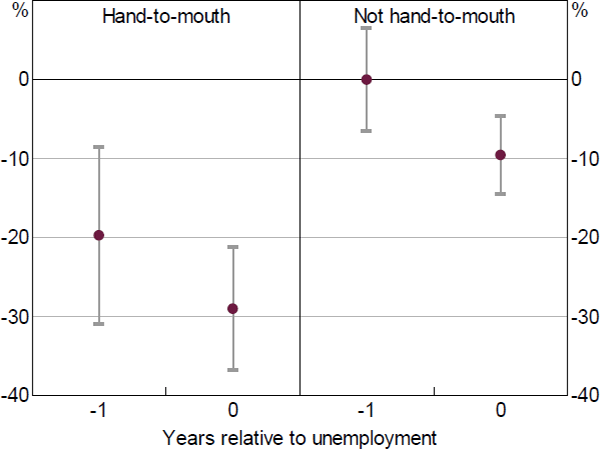
For this, we estimate the model separately for liquidity-constrained households and all other households. We find that liquidity-constrained households reduce spending by more than other households in response to unemployment (Figure 13). Interestingly, liquidity-constrained households also reduce spending in the year before unemployment. This is consistent with liquidity constraints being an important part of the story. It also highlights that even asset-rich households may experience large consumption losses due to illiquid wealth. Households that are not liquidity constrained also reduce spending in response to unemployment.
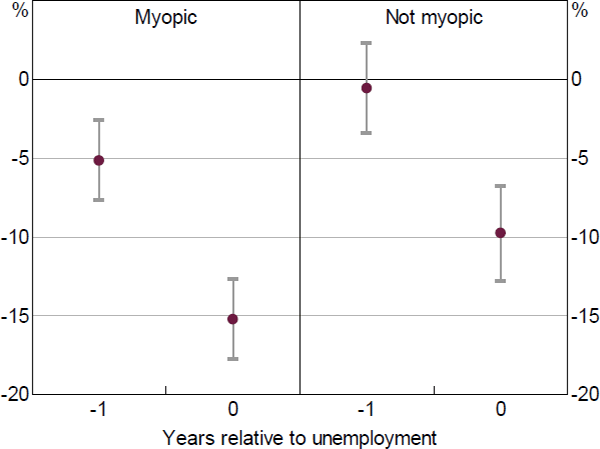
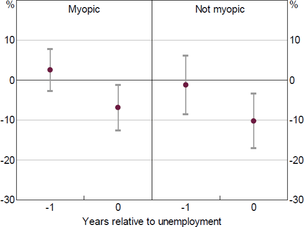
We follow the same sub-sampling approach to test whether myopic households are more sensitive to unemployment in their spending response. We measure myopia based on responses to a specific question about the time frame in which each household plans saving and spending decisions. A household is considered myopic if the most important time frame is one year or less. On this metric, we find no difference between the spending responses at the onset of unemployment for myopic households compared to forward-looking households (Figures 14 and 15).
Note: Lines represent 95 per cent confidence intervals
Sources: Authors' calculations; HILDA Survey Release 19.0
Note: Lines represent 95 per cent confidence intervals
Sources: Authors' calculations; HILDA Survey Release 19.0
Note: Lines represent 95 per cent confidence intervals
Sources: Authors' calculations; HILDA Survey Release 19.0
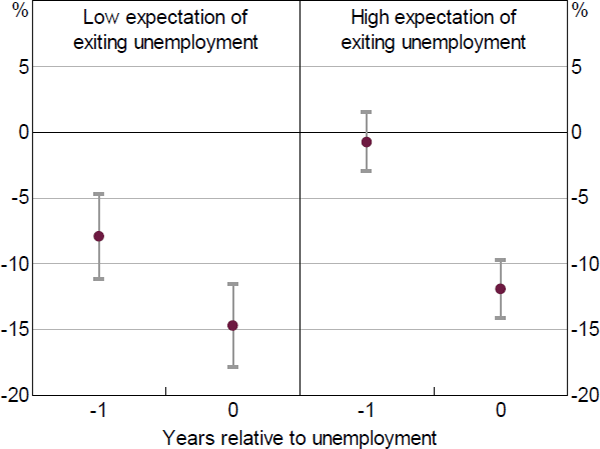
We also test whether, during unemployment, the consumption response varies by how long individuals expect to remain unemployed. To do this, we follow the same approach but split household heads into low (high) expectations of regaining work based on whether their expected probability of regaining work in the year ahead is below (above) 75 per cent (which is the mean response). We find larger consumption losses for unemployed workers that do not expect to regain employment within the year relative to those that do (Figures 16 and 17). This is consistent with these households smoothing consumption through a period of unemployment. However, these differences are not statistically significant.
Note: Lines represent 95 per cent confidence intervals
Sources: Authors' calculations; HILDA Survey Release 19.0
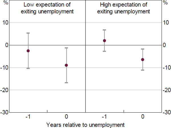
Note: Lines represent 95 per cent confidence intervals
Sources: Authors' calculations; HILDA Survey Release 19.0
Footnotes
We find other sources of heterogeneity in the spending response to job loss, including personal characteristics such as age and income. The effect of job loss on spending varies with age. Specifically, it appears to be a quadratic function of age, with households where the head is aged 45 to 54 most sensitive to unemployment. Two factors may drive this relationship. First, younger households have more time over which to smooth the earnings losses from unemployment. Thus the PIH would imply that they respond less to earnings losses. Second, older households are less likely to be liquidity constrained, and as a result more able to smooth the effect of unemployment. The effect of job loss on spending also varies with the level of household income. Low-income households experience the largest reductions in spending. This is consistent with low-income households being more liquidity constrained. However, even high-income households reduce spending in response to job loss. [17]
We also tested whether job loss expectations affect spending in the modelling framework of Stephens (2004). We found similar results in that there is no evidence that anticipated job losses affect spending. We also tested all the spending regressions with a Poisson fixed effects model instead of a log linear model and the results were unchanged. [18]
As the hand-to-mouth variable is constructed using variables only available in the wealth module, and total expenditure is only available for a small subset of the sample, we are unable to estimate the total expenditure response to unemployment by hand-to-mouth status. [19]
Under the Kaplan et al (2014) framework, households are considered ‘hand-to-mouth’ if their fortnightly income is greater than or equal to their current liquid net wealth. [20]