RDP 2021-08: Job Loss, Subjective Expectations and Household Spending Appendix A: Testing the Predictive Ability of Workers' Subjective Expectations
August 2021
- Download the Paper 2,109KB
Here, we outline a simple model of expectations formation to more formally test the predictive ability of workers' subjective expectations. As well as testing whether subjective expectations contain predictive information for job loss above other observable variables, we examine whether worker expectations are fully rational, or whether their mistakes are systematic and predictable.
There is a significant body of literature in macroeconomics that tests the predictions of the workhorse model of expectations formation – the full information rational expectations (FIRE) hypothesis. There is also a large body of labour market research that studies the role of subjective expectations about employment. But there have been few studies that link these 2 lines of research. Most of the macro research has focused on surveys, typically of professional forecasters, and on how well they forecast aggregate variables like GDP growth and inflation. The studies on subjective expectations usually focus on the ability of individual workers to predict their own employment outcomes, but are less interested in what this tells us about how consumers form expectations and what this means for the macro economy. There are advantages to combining these 2 approaches using longitudinal data.
We adapt the framework of Keane and Runkle (1990) that tests the FIRE hypothesis based on a survey of professional forecasters. Expectations are assumed to be rational if they are equal to mathematical expectations conditional on the set of all information relevant to the worker. For an individual worker, we can express this relationship as:
Which states that the worker's expectation of employment next year is their (one-year-ahead) prediction of actual employment ( yit+1 ) based on the information set available to them at the time of the survey . This is equivalent to the statement expressed in terms of forecast errors:
For an individual worker the test of rationality involves running the regression:
where the dependent variable is the ‘true’ probability of job loss for worker i in survey year t + 1. In practice, the researcher does not observe the ‘true’ probability of job loss – we only observe the ex post binary outcome of whether a worker lost their job or not.
It is possible that beliefs about job prospects evolve differently across individuals over time. To allow for this, the equation also includes a set of control variables ( Xit ) for factors that may affect their willingness and ability to predict future job outcomes at a given point in time, such as the worker's age, sex, job tenure and industry of work.
The key explanatory variable is the worker's estimated probability of job loss in year t +1 as surveyed in year t. Under rational expectations, the estimated intercept should be zero , the slope coefficient on the subjective expectations should be equal to unity and the slope coefficients on the vector of control variables should be zero . Note that rational expectations allows individuals to hold different beliefs if they have different information sets (i.e. private information).
As Keane and Runkle (1990) argue, OLS estimates of the equation are likely to be biased. This is because the forecast errors across individuals could be correlated at a point in time (for example, because of an aggregate shock that affects job security in their industry). To partly address this, we specify the error term such that it includes both a worker fixed effect and an aggregate time fixed effect :
This simple adaption of the model provides a useful test of how worker expectations are formed. By including an individual worker fixed effect we allow for the possibility that an individual's forecast errors are correlated with an individual's time-fixed private information (e.g. previous forecast errors or their inherent ability). Because we have longitudinal information on individual workers and they are predicting their own outcomes, we can also test whether workers make systematic errors in aggregate. We do this by including time fixed effects. Many macro studies cannot follow this approach because the dependent variable is an aggregate variable being predicted by a range of forecasters at a specific point in time. The inclusion of time fixed effects would lead to perfect collinearity with the dependent variable, so the model could not be estimated.
We estimate the model above and test the FIRE hypothesis using 2 modelling approaches. The first approach is to estimate a linear probability (OLS) model for actual job loss on job loss expectations with (and without) individual worker fixed effects and controls. The second approach estimates a logistic regression because job loss is a binary outcome. The results of estimating Equation (A1) under the various approaches are shown in Table A1.
| OLS | OLS | Fixed effects | Logit | |
|---|---|---|---|---|
| Without controls | With controls | With controls | With controls | |
| Expected job loss | 0.18** (33.74) |
0.17*** (30.85) |
0.15*** (24.78) |
0.09*** (39.34) |
| Household fixed effects | No | No | Yes | No |
| Year fixed effects | No | Yes | Yes | Yes |
| R squared | 0.03 | 0.05 | 0.27 | 0.11 |
| Joint test (F-statistic) | F (1, 17,512) = 1,138.4 |
F (116, 17,378) = 19.7 |
F (115, 17,378) = 9.2 |
na |
| Observations | 114,822 | 111,806 | 111,806 | 111,806 |
|
Notes: ***, ** and * denote statistical significance at the 1, 5 and 10 per cent levels, respectively; standard errors are clustered by household, with t-statistics in parentheses; estimated coefficients on individual worker and year fixed effects not shown; regressions in columns 2 to 4 include control variables for demographics, such as age and education, and past labour force status, such as job tenure and the industry of work; see Appendix B for the full regression output; the joint test is a test that all the coefficients on the explanatory variables are jointly equal to zero Sources: Authors' calculations; HILDA Survey Release 19.0 |
||||
The results indicate that workers' subjective job loss expectations have some ability to predict actual job loss in the year ahead. Indeed, subjective expectations contain predictive power over and above the information observed by the econometrician about the worker. In each model specification, the regression coefficient on expected job loss is positive and significantly different from zero. A 1 percentage point increase in the expected probability of job loss is associated with an increase of about 10 to 18 basis points in the actual probability of job loss. This economic effect is small and t-tests confirm it is far from the value of one, pointing to a violation of rational expectations. These results are robust to changes in model specification, including the addition of lags on subjective expectations, and controlling for subjective response ‘bunching’ by including dummies for whether expectations are 0, 50 or 100 per cent. The inclusion of worker fixed effects causes the coefficient estimate for expected job loss to fall slightly (comparing columns 2 and 3 of Table A2). This points to a significant and correlated worker-specific component in both the true and expected probability of job loss.
We can also estimate the same model to test whether unemployed workers' expectations of job finding have predictive power for actual job finding rates. The results are shown in Table A2. Here, the sample is restricted to unemployed workers.
| OLS | OLS | Fixed effects | Logit(a) | |
|---|---|---|---|---|
| Without controls | With controls | With controls | With controls | |
| Expect to find employment within a year |
0.29*** (47.63) |
0.24*** (33.44) |
0.12*** (12.56) |
0.25*** (31.95) |
| Household fixed effects | No | No | Yes | No |
| Year fixed effects | No | Yes | Yes | Yes |
| R squared | 0.09 | 0.12 | 0.03 | 0.16 |
| Observations | 23,985 | 22,660 | 22,660 | 22,660 |
|
Notes: ***, ** and * denote statistical significance at the 1, 5 and 10 per cent levels, respectively; standard errors are clustered by household, with t-statistics in parentheses; estimated coefficients on year fixed effects not shown; regressions in columns 2 to 4 include control variables for demographics, such as sex, age and education; see Appendix B for the full regression output (a) Marginal effects Sources: Authors' calculations; HILDA Survey Release 19.0 |
||||
Again, expectations hold significant predictive power for future labour market outcomes. The subjective expectation of finding a job within the next 12 months is positively correlated with the actual rate of job finding over the period. This holds true even when we control for a range of worker characteristics, such as age and past labour force status. Notably, the inclusion of worker fixed effects causes the coefficient estimate to halve in size, which is again consistent with a fixed component to both expectations and realised unemployment duration, and indicates that individuals are good at predicting unemployment duration risk both overall and over time.
We can also exploit the longitudinal nature of the household-level data to examine how expectations of job loss evolve in the years just before and after a job loss event. To do this, we specify a model of job loss expectations with controls for time and individual fixed effects, and plot estimated coefficients on leads and lags of actual job loss. Using a fixed effects framework allows us to extract the component of job loss expectations that is correlated with a specific job loss event. We find that, for workers that lose their jobs, their subjective estimates of job loss rise in the 2 years leading up to the event (Figure A1).
This suggests that, despite evidence of bias, workers can predict actual labour market outcomes, even a few years out from the event. We also find that job loss expectations remain elevated in the year of the event, but one year later return to the same level as they were before the event.[21] This implies that there is no permanent change to individuals' job loss expectations following a job loss event.
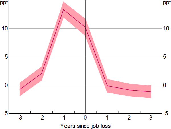
Notes: Estimates are obtained from a linear fixed effects regression that includes year dummies; shaded area is 95 per cent confidence interval
Sources: Authors' calculations; HILDA Survey Release 19.0
Footnote
We are able to elicit job loss probabilities from respondents in the year of job loss (year t ) since the majority of those who lost their job go on to regain employment before the time of the survey. [21]