RDP 2018-07: The GFC Investment Tax Break 5. RD with BLADE
June 2018
- Download the Paper 1.8MB
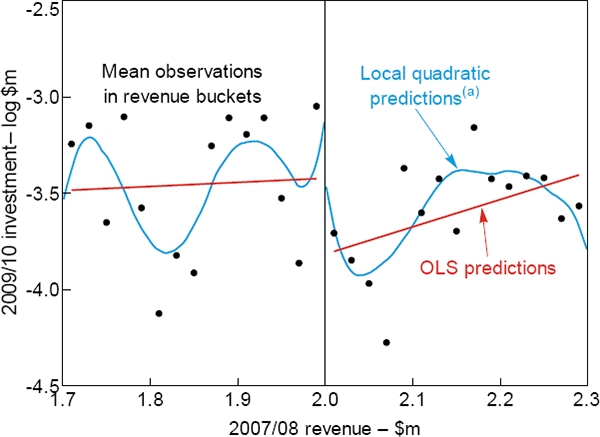
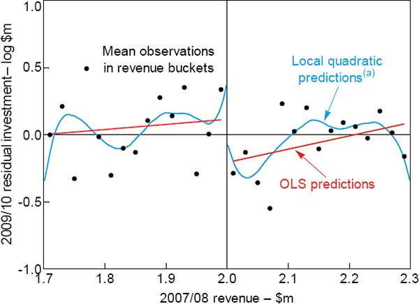
Before outlining the formal model, we provide a graphical version of the RD analysis. Figure 3 plots log investment against revenue in 2007/08. The dots represent the mean investment by businesses falling into different revenue buckets ($20,000 wide). The red and blue lines are lines of best fit, estimated separately for businesses above and below the $2 million threshold using a linear (OLS) model and a local quadratic polynomial, respectively. All three provide evidence of a sizeable fall in investment at the threshold, indicating that the tax break affected investment. This is even clearer if we plot the residuals from a regression of investment on industry dummies, instead of investment itself, which accounts for the fact that businesses in certain industries are likely to invest more heavily (Figure 4).

Note: (a) Modelled using Epanechikov kernel with a bandwidth of 0.05

Notes:
Residual investment is from regression of log investment in 2009/10 on industry fixed effects
(a) Modelled using Epanechikov kernel with a bandwidth of 0.05
5.1 Econometric Methodology
In an RD model, the estimate of the effect of the treatment, β, is taken as the difference between the conditional mean just below the threshold and the conditional mean just above the threshold. That is:
where βRD is the regression discontinuity estimate, Yi is the variable of interest, Xi is the forcing variable and c is the threshold.
The problem can be thought of as estimating a local polynominal model on either side of the threshold to estimate the conditional means. This leads to three modelling choices:
- Bandwidth: This determines whether observations a long way away from the point of interest are included in the regression. A high bandwidth means we include observations a long way away from the threshold, whereas a low bandwidth means we focus only on near observations. Bandwidth choice amounts to weighing up bias, which increases with the bandwidth as we are including observations far away from the point of interest, with efficiency, which rises with the bandwidth as we are including more observations and getting more information. We choose a bandwidth of $270,000 based on the mean squared error minimising plug-in estimator of Imbens and Kalyanaraman (2012).
- Kernel choice: The choice of kernel determines the weights different observations are given in the polynomial regression. We use a rectangular or uniform kernel, which gives equal weight to all observations and amounts to only including observations within the bandwidth (i.e. revenue in 2007/08 between $1.73 million and $2 million for the conditional mean below the threshold, and between $2 million and $2.27 million for the conditional mean above).
- Polynomial order: This is the order of the polynomial in the forcing variable that is used to fit the data. A higher-order polynomial will more flexibly fit the data, especially if we have to use a high bandwidth due to a lack of observations around the threshold. However, increasing the order of the polynomial could lead to overfitting. We focus on a polynomial of order 1 (i.e. a linear model). We use the test suggested by Lee and Lemieux (2010) and find this is sufficient for our baseline bandwidth.[14]
Appendix B provides robustness testing around these modelling choices.
Given these modelling choices, our RD model is:
where the business identifier is i, t is the year 2009/10, and I is an indicator variable that takes on the value 1 if the condition in the brackets is met. The coefficient of interest, β, captures the discontinuity at the revenue threshold. A significant and positive estimate for this coefficient would indicate that the higher tax break led small businesses to invest more.
As we model the log of investment, any observation of zero investment is discarded. This accounts for a non-negligible portion of the sample. As such, the estimates are estimates of the effect of the tax break on businesses' investment at the intensive margin (i.e. how much they invest, conditional on investing). We use the log of investment, instead of levels, as this enables us to compare our estimates to the semi-elasticities reported in the existing literature.
5.2 Baseline Results
Table 3 shows the results from this baseline model.[15] Model 1 is the model outlined in the previous subsection. Models 2 and 3 incorporate some additional covariates, namely revenue in period t and t − 1, and ANZSIC division dummies.[16] While the RD approach does not require the inclusion of covariates, doing so can increase the efficiency of the estimates and help to eliminate small sample biases (Imbens and Lemieux 2008). Finally, Models 4 and 5 present the results from estimating the model using a polynomial of order 2 (i.e. a quadratic) in Revenuei,t − 2. Calonico, Cattaneo and Titiunik (2014) suggest that this is a simple way to account for asymptotic bias introduced by standard bandwidth selection methods, which tend to be too ‘large’ in asymptotic terms.[17]
| Model | |||||
|---|---|---|---|---|---|
| 1 | 2 | 3 | 4 | 5 | |
| β | 0.49** (0.19) |
0.50*** (0.19) |
0.49*** (0.19) |
0.71** (0.28) |
0.77*** (0.28) |
| Controls | |||||
| δ1 | 2.36*** (0.80) |
2.22*** (0.80) |
2.41*** (0.78) |
3.40 (1.16) |
4.64 (3.22) |
| δ2 | −1.94 (1.32) |
−1.46 (1.33) |
−1.76 (1.31) |
1.16 (4.94) |
0.35 (4.85) |
| Revenuei,t | na | 0.29** (0.14) |
0.33** (0.16) |
na | 0.34** (0.17) |
| Revenuei,t − 1 | na | 0.26 (0.42) |
0.16 (0.42) |
na | 0.13 (0.43) |
 |
na | na | na | −3.81 (11.42) |
−8.18 (11.32) |
 |
na | na | na | 19.89 (18.02) |
25.11 (17.64) |
| Dummies | None | None | Division | Division | Division |
| Bandwidth ($m) | 0.27 | 0.27 | 0.27 | 0.27 | 0.27 |
| Kernel | Uniform | Uniform | Uniform | Uniform | Uniform |
| Observations | 1,245 | 1,228 | 1,228 | 1,245 | 1,228 |
|
Notes: ***,**,* represent statistical significance at the 10, 5 and 1 per cent significance levels, respectively; standard errors are in parentheses |
|||||
The estimated treatment effect, β, is positive and significant in all models. Most of the estimates are around 0.5, indicating that qualifying for the higher rates of tax break available to small businesses caused businesses to invest around 65 per cent more. Using the average difference in tax break rates over 2009/10 of 20 percentage points, this translates into a semi-elasticity of investment with respect to the tax break rate of 3.25 (i.e. a 10 percentage point increase in the tax break raises investment by about 33 per cent). Given the expiry of the credit was known in advance, meaning that businesses may have brought their investment forward to the first half of the year, it is also reasonable to treat the average difference for the full year as that prevailing over the first half of 2009/10: this would give a semi-elasticity of 1.63.
Given our assumption that the tax break does not affect the user cost of capital for companies in our sample, we interpret this strong response as indicating that the tax break influences company investment through some other mechanisms. As discussed above, one potential mechanism is the relaxation of financial constraints.
The fact that we find evidence of a role for other mechanisms is consistent with ZM's finding that businesses in their sample respond more strongly when they are tax profitable, such that investment deductions reduce their current year tax, or when they are more financially constrained.
Still, these estimated elasticities are somewhat smaller than those from ZM. ZM provide a baseline semi-elasticity for their sample of 3.7, but this is estimated using a sample of companies that are mostly much larger than our RD sample (median revenue in their dataset is $26 million). Their estimate for the bottom three deciles of their sample, which are more comparable in size to our sample, is 6.3. The fact that companies in the United States respond more strongly to tax breaks than Australian companies is consistent with the difference in taxation arrangements. The United States has a classical company taxation regime whereby company dividends are subject to individual income taxes, so company tax deductions are valuable to shareholders.[18] The fact that we use total capital expenditure instead of equipment expenditure could also help to explain why our estimated coefficients are below those for the United States, as the additional noise would introduce a downwards bias. However, given we focus on small businesses that are unlikely to frequently engage in building investment, we think this bias will be very small.
The RD approach also allows us to test whether the increased investment in response to the tax break was merely brought forward from future years, or whether it represented an actual increase in the total amount of investment, and therefore the capital stock. In the former case, we would expect lower investment from small businesses in later years to make up for the higher investment in 2009/10.
We can test for this by replacing the left-hand side variable with investment in 2010/11, or in 2011/12, or the sum of the two. The results from doing so, using the specification from Model 2, are contained in Table 4. There is no evidence of lower future investment for small businesses, indicating that the investment tax break generated genuine additional investment, rather than simply bringing forward investment. This is consistent with the findings in HS and ZM. The results are robust to the choice of controls, and to re-selecting the optimal bandwidth.
| Investment for year | |||
|---|---|---|---|
| 2010/11 | 2011/12 | 2010/11–2011/12 | |
| β | 0.21 (0.22) |
0.15 (0.21) |
0.12 (0.40) |
| Dummies | None | None | None |
| Bandwidth ($m) | 0.27 | 0.27 | 0.27 |
| Kernel | Uniform | Uniform | Uniform |
| Observations | 1,150 | 1,088 | 903 |
|
Notes: Uses Model 2 from above; standard errors are in parentheses |
|||
5.3 Validity Testing
5.3.1 Placebo tests
The above results indicate that qualifying for small business status led these businesses to invest significantly more in 2009/10. One concern is that this may be unrelated to the tax break itself. There are, for example, a number of other tax concessions that were available to small businesses at the time that could have caused businesses to invest more if they were considered small for tax purposes. These include reduced taxation of capital gains, accelerated depreciation for assets worth less than $1,000, income and sales tax concessions for businesses with revenue below $75,000, and reductions in intra-year tax instalments. A table detailing these policies is provided in Appendix D.
Most of these concessions were in place prior to the financial crisis or remained in place after 2009/10. As such, if they are substantially affecting our results in 2009/10, their effect should also be evident during other years. In contrast, the effect of the tax break should only be evident in 2009/10, and possibly in 2008/09 given the tax break rate differed for the final month and a half of this year. This suggests the natural placebo test of re-running our RD model using data for other years.
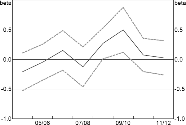
We perform the placebo testing using Model 2 from above, but the results are robust to other choices. Figure 5 plots the estimated treatment effects and confidence bounds. For all years with no tax break, the treatment effect is not statistically significantly different from zero. For 2008/09, the treatment effect is significant and is estimated to be around half the size of that in 2009/10. The fact that we find a significant effect despite the relatively short portion of 2008/09 during which the tax break rates differed suggests that firms placed a high value on receiving the tax benefit immediately, rather than waiting to receive the benefit at the end of the next tax year.

Notes: Estimated using Model 2; dashed lines are 95 per cent confidence intervals
Placebo tests can also be used to test for confounding factors that were only present during 2009/10. For example, while we are not aware of any relevant tax rules that differed by size and applied only in the years we investigate, such differences may have escaped our notice. The appropriate tests examine whether other observables that are less likely to be affected by the treatment are continuous in the forcing variable. We examine both revenue in 2009/10 and full-time equivalent employment. Using a specification based on Model 1, we find no evidence of a discontinuity.[19]
5.3.2 Manipulation tests
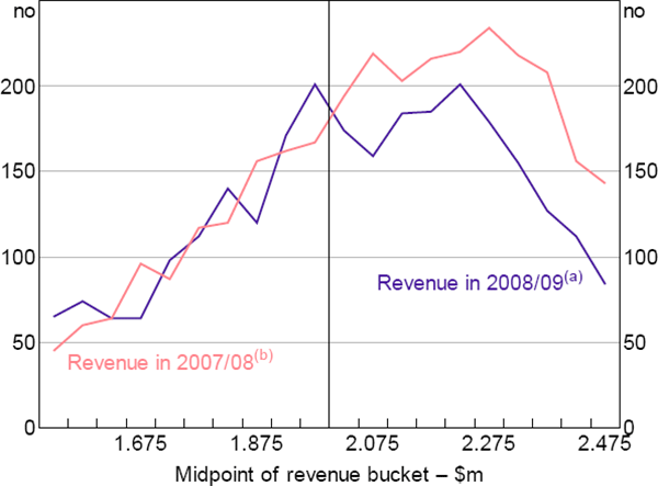
One of the requirements for valid RD is that businesses cannot manipulate the forcing variable, Revenue, to change their treatment status. If businesses could self-select in this way, the assumption that businesses just above and below the cut-off are identical would be violated. Businesses with a higher ex ante propensity to invest would have a greater incentive to select into treatment. In our case, manipulation of the forcing variable – revenue measured about a year before the announcement of the differential tax break – is improbable. Consistent with this, there is no graphical evidence of bunching of businesses just below $2 million of revenue in 2007/08, which we would expect to see if businesses were lowering revenue to get under the threshold (Figure 6). Applying the formal test suggested by Cattaneo, Jansson and Ma (2017) confirms this finding.

Notes:
Buckets are $50,000 wide
(a) Businesses with revenue in 2007/08 between $1.73–2.27 million
(b) Businesses with revenue in 2008/09 between $2–2.5 million and revenue in 2009/10 above $2 million
One additional concern that is fairly unique to our RD set-up is that businesses might be manipulating their way out of the estimation sample. In particular, businesses with revenue above $2 million in 2007/08, and who forecast revenue just above $2 million in 2008/09 or 2009/10, might have the incentive to manipulate their revenue in those years to qualify for the tax breaks. Based on our inclusion criteria, these businesses will drop out of our estimation sample. Moreover, businesses with a higher propensity to invest would have a greater incentive to manipulate their revenue. This would cause our sample of large businesses to have a lower propensity to investment, compared to the ‘true’ population.
There is some evidence of businesses manipulating revenue in 2008/09 to get below the threshold, with a spike in the number of businesses with revenue just below the threshold. This provides further evidence that the tax breaks were valuable to companies, as otherwise there would be no reason to manipulate their revenue. But it does suggest that there may be some threat to the validity of our identification strategy, even if the number of businesses that appear to manipulate is small relative to the total sample size.
One way to test whether our samples of small and large businesses are different is to test whether pre-determined covariates are continuous in the forcing variable. If businesses either side of the threshold really are identical apart from the treatment, their pre-determined covariates should also be identical. We test this using investment in 2007/08, before the introduction of the investment tax break, and find no evidence of a discontinuity. In the parlance of the RD literature, the density of investment in 2007/08 appears to be continuous at the threshold. This suggests the two samples do not have differing propensities to invest and supports the validity of the RD approach.
Still, even if businesses either side of the threshold had similar propensities to invest in 2007/08, it does not mean that this would necessarily be the case in 2009/10. To account for this, we rely on the fact that businesses are only likely to be able to manipulate their revenue to a certain extent. Businesses with revenue just above $2 million will likely be able to manipulate their revenue down, but businesses with revenue well above $2 million could not. As such, manipulation out of the sample, and therefore a potentially downwardly biased propensity to invest, should only be an issue for large businesses with revenue in 2008/09 and 2009/10 just above $2 million.
Table 5 contains the results from removing businesses with revenue between $2 million and $2.1 million in 2008/09 and 2009/10 from the sample. While somewhat arbitrary, the choice of a $100,000 ‘buffer’ range is supported by Figure 6. Models 6 and 7 show the results using the same bandwidth as in our baseline model, while Models 8 and 9 show the results using the automatic bandwidth selection and bias adjustment of Calonico et al (2014).
| Model | ||||
|---|---|---|---|---|
| 6 | 7 | 8 | 9 | |
| β | 0.53** (0.24) |
0.57** (0.24) |
0.45** (0.23) |
0.54** (0.23) |
| Controls | None | Revenue | None | Revenue |
| Bandwidth ($m) | 0.27 | 0.27 | 0.38 | 0.36 |
| Kernel | Uniform | Uniform | Triangular | Triangular |
| Observations | 899 | 885 | 2,371 | 2,317 |
|
Notes: Sample excludes businesses with revenue in 2008/09 or 2009/10 between $2 million and $2.1 million; ***,**,* represent statistical significance at the 10, 5 and 1 per cent significance levels, respectively; standard errors are in parentheses |
||||
Using the same bandwidth, the estimated treatment effects are broadly the same as in the baseline specification, though the point estimates are slightly higher. However, once we re-select the bandwidth, we get point estimates that are slightly below our baseline estimates. Nevertheless, the difference in the estimates is small and not statistically significant, suggesting that the fact that businesses are manipulating out of our sample is not substantially biasing our baseline estimates.
Footnotes
They suggest including a full set of bin dummies in the regression, and jointly testing whether the coefficients are zero. The advantage of this approach is that it would also pick up other discontinuities in investment. [14]
Clustering the errors by 4-digit ANZSIC group leads to slightly higher p-values, but does not change the significance of the results. [15]
Unless the covariates have very high explanatory power, their inclusion should not affect the optimal bandwidth (Imbens and Kalyanaraman 2012). As such, we use the same bandwidth for these models. [16]
We also tried using their bandwidth selection rules and variance estimator, as implemented using the Stata ‘rdrobust’ package. The estimated treatment effects were generally around 0.5–0.6 across a number of specifications with different kernels and covariates. [17]
Some US corporates (S corporations) are taxed on a pass-through basis akin to the treatment of unincorporated businesses in Australia. [18]
The latter also suggests that businesses did not ‘fund’ the investment by substituting away from labour. This is broadly consistent with the findings in ZM, though they actually find that employment increased. [19]

