RDP 2018-07: The GFC Investment Tax Break 4. Data and Methodology
June 2018
- Download the Paper 1.8MB
This section explains the two different methodologies and two different datasets that we use to measure the effect of the tax break.
4.1 RD with BLADE
The definition of a small business lends itself to RD methods. This is because whether or not a business is small (the treatment), and therefore the level of the tax break, depends on whether a continuous ‘forcing’ variable (revenue in past years) is above or below a threshold ($2 million). Our RD set-up looks at investment for businesses with revenue just above the threshold, and those with revenue just below the threshold, and takes the difference to be the effect of the treatment. The underlying assumption is that businesses just either side of the cut-off will be nearly identical along all relevant dimensions, except for the size of the tax break. Under certain assumptions – including that the businesses cannot manipulate revenue and so self-select into treatment – treatment is as good as randomly assigned and the approach is equivalent to a randomised experiment.[9] This is the approach we take in Section 5.
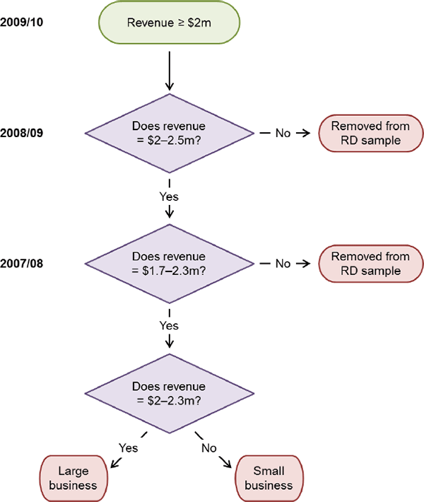
Establishing a clean regression discontinuity requires us to focus on a subset of businesses. For the RD analysis, we focus on 2009/10, which we refer to as time t. This is the year in which the difference in the tax break for small and large businesses was at its largest.[10] We further limit the dataset to businesses with revenue above $2 million in 2008/09 (t − 1). Based on the tax rules, these businesses could qualify as small businesses only if:
- their revenue in 2009/10 (measured at the end of the year) was below $2 million; or
- they had revenue below $2 million in 2007/08 (t − 2) and they expected revenue in 2009/10 to be below $2 million.
As condition (a) provides a possible way to manipulate treatment, we drop any businesses with revenue in 2009/10 below $2 million from the sample. Condition (b) then provides an appropriate forcing variable for our subset of businesses: revenue in 2007/08. The remaining businesses in the sample were large if their revenue in 2007/08 was above $2 million. Otherwise, they were small businesses, provided they could reasonably expect their revenue in 2009/10 to be less than $2 million.
To deal with this expectational requirement, we further exclude businesses in 2008/09 with revenue above a ceiling. We do so because revenue in the previous year is one of the most relevant considerations when projecting current year revenue (ATO 2017b), and so businesses with revenue above a ceiling in the previous year would be unlikely to be able to argue that they are small. Setting the ceiling too high would mean that we treat some large businesses as small businesses and, under the maintained hypothesis, this would bias our estimates down. Setting the ceiling too low would mean that we are throwing away useful observations and would lead to a loss of efficiency. We choose a ceiling of $2.5 million. While somewhat arbitrary, the results are robust to the choice of ceiling (see Appendix B).
Figure 2 provides a visual representation of this selection rule. We are left with businesses with: revenue in 2008/09 between $2 million and $2.5 million; and revenue in 2009/10 above $2 million. We then focus on a subset of businesses with revenue in 2007/08 within an interval around the $2 million threshold (we discuss the selection of this ‘bandwidth’ in Section 5.1).
We apply RD methods to a dataset derived from the ABS's BLADE (Hansell and Rafi 2018). This dataset contains administrative tax data for almost the entire population of Australian companies and unincorporated businesses.[11] The size of this dataset makes it ideally suited to the RD approach, which requires enough observations close to the threshold to form an estimate of the effect (once we have applied the trimming discussed above).
Our RD results with the BLADE data provide our most robust estimate of the causal effect of the investment tax break upon investment. But some elements of this approach are unsatisfactory. First, the BLADE data only contains data on aggregate building and equipment investment, while the tax break applied only to the latter.[12] This means that we are estimating the response of total investment to an equipment investment tax break when using BLADE. Second, despite its large size, once we narrow the BLADE sample sufficiently to run our RD model there almost no unincorporated businesses left. As such, the approach provides estimates for companies only and does not allow us to check for heterogeneous responses across business types. Finally, the treatment effect estimated using RD is very local, as it only tells us about the effect of the treatment for businesses with revenue close to the threshold, and even then only businesses that have a revenue path that meets our trimming rules (i.e. that grow somewhat year-to-year). The response to the tax break for these businesses might differ from that of businesses of different sizes and growth paths.
4.2 DD with Capex Survey Data
Our second dataset – business-level data from the ABS's Survey of New Capital Expenditure (Capex Survey) – allows us to address some the weaknesses of the RD analysis. This survey seeks responses from around 9,000 businesses each quarter, and is used to estimate quarterly population-level capital expenditure (capex) aggregates for Australia. It separates equipment and building investment, which allows us to concentrate on equipment investment, and to run a placebo test using (ineligible) building investment. An additional advantage is that we can work with population-level data by applying sampling weights. This approach allows us to easily estimate an aggregate response to the tax break, and evaluate its macroeconomic importance.
The dataset has two key drawbacks. First, the Capex Survey dataset does not allow us to measure past revenue as precisely as in BLADE due to sample rotation. As such, we take the simple approach of designating businesses with revenue below $2 million in the financial year prior to the current quarter as small, and all other businesses as large. This is an approximation of the detailed eligibility rules discussed above. The second key drawback of this dataset is that we cannot use RD methods – it does not have sufficient observations in the vicinity of the threshold.
Instead we apply a DD model to the Capex Survey data. This approach relies on identifying a control group (large businesses) and a treatment group (small businesses). It measures the effect of the tax break as the difference between the change in investment for the treatment group across the treatment and non-treatment periods, and the change for the control group across the two periods. The key assumption underlying this approach is that in the absence of treatment, the control group and the treatment group would have behaved similarly (the parallel trends assumption).
The causal identification in the DD model is likely to be weaker than in the RD model. This is because the parallel trends assumption is a much stronger assumption than that used in RD. Still, we present evidence below that the parallel trends assumption is satisfied, particularly for our preferred control group of businesses with lagged revenue between $2 million and $10 million.
Moreover, because of the less data-intensive nature of DD, it allows us to examine heterogeneity across business types and sizes.[13]
Footnotes
For discussions of the theory and practice of the RD approach, see, for example, Imbens and Lemieux (2008) and Lee and Lemieux (2010). [9]
The tax break also differed for the final 1.5 months of 2008/09. We discuss this in Section 5.3 below. [10]
Businesses not registered for the goods and services tax (GST) are not included in the dataset. Very small businesses, that either never have sales above $75,000, or that never employ a worker, are removed from the dataset. [11]
For details on the particular data we use, see Appendix A. [12]
We could estimate a DD model using the BLADE data to examine these heterogeneities. But we prefer to use the Capex Survey given it differentiates between investment types and is available at a quarterly frequency, which allows us to exploit quarter-to-quarter variation in the deduction rates. BLADE data are only available at an annual frequency. [13]