RDP 2015-14: Okun's Law and Potential Output 5. Forecasting

An important problem confronting macroeconomic policymakers – and a motivation for this paper – is that unemployment forecasts have been biased. For example, since 2000 the unemployment rate has, on average, been 0.22 percentage points lower than the RBA staff forecast it to be one year earlier. This is difficult to attribute to chance; the hypothesis that the forecasts are unbiased can be rejected with a p-value of 4 per cent.^[8] This bias has been a recurring feature of the RBA forecasts, also being statistically and economically significant in data from the 1990s. Tulip and Wallace (2012) discuss this further.

The bias in the unemployment forecast is not due to low GDP forecasts. Since 2000, the RBA's forecasts of real GDP growth have actually been too high (the wrong sign to explain unemployment bias), whereas over the 1993–2011 sample reported by Tulip and Wallace (2012, Table 4), they have been unbiased.

One possible explanation for this discrepancy is that forecasters are doing a reasonable job in forecasting actual output growth, but when they translate that into unemployment, they use an out-of-date estimate of potential output growth. They may not realise that larger declines in unemployment are likely to accompany a given growth rate of GDP than in the past.

To assess this, we examine the pseudo real-time forecasting performance of our constant coefficients and time-varying coefficients models and compare this with the actual real-time forecasts of the unemployment rate by the RBA. For each quarter t, we estimate our models up to quarter t − 1, from which we take coefficients and the latest estimates of state variables.^[9] We combine these with real-time RBA forecasts of GDP growth for quarters t, t + 1, …, t + h to project right-hand side variables, and then forecasts of the unemployment rate through to t + h. An important assumption underpinning this exercise is that the RBA forecasts of output growth are independent of changes in our estimate of potential GDP growth. We then repeat for quarter t + 1 and so on, giving us sequences of forecasts at each horizon.

We attempt to estimate our models on the data available to forecasters at the time. Real-time data and forecasts for the unemployment rate and GDP growth are described in Tulip and Wallace (2012), which we have updated. We do not have access to real-time vintages of the change in real unit labour costs, so we use the 2015 vintage of data for quarters before the forecast and assume zero change in real unit labour costs for quarters t, t + 1, …, t + h. The use of revised data may give rise to concerns that we may overstate our model's forecasting performance at short horizons. However, including real unit labour costs actually reduces the model's forecasting performance over the sample we use (the explanatory power of this variable comes from the 1970s and 1980s).

We focus on a subset of the available data that we think is most informative. Our evaluation period begins in 2000, given the availability of forecast information. As discussed below, some of our conclusions are sensitive to this choice. We show results for horizons out to six quarters ahead. We have a smaller sample of longer-term forecasts, which is heavily influenced by the global financial crisis, and we suspect is unrepresentative. Moreover, it is less plausible to take longer-term output growth forecasts as given when varying potential output assumptions.

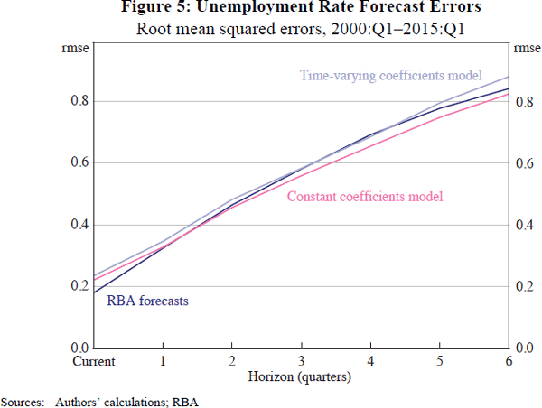
Forecast comparisons are shown in the figures below. Figure 5 shows root mean squared errors, a standard measure of forecast accuracy. By this metric, all three forecasts perform similarly. Differences are not economically or statistically significant (judging by Diebold-Mariano tests, not shown).

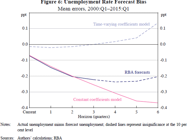
Figure 6 shows mean errors, a measure of bias. Solid lines are significantly different from zero at a 10 per cent level. The precision (though not the magnitude) of estimates tends to decline as the horizon increases, as we have fewer independent observations. Whereas the RBA and constant coefficients forecasts are noticeably biased, the bias in the time-varying coefficients forecasts is insignificant, in either statistical or economic terms.

The favourable performance of the time-varying coefficients forecast is surprising and important. The relationship between output and unemployment is often described in complicated structural terms (Layard, Nickell and Jackman 1991; Debelle and Vickery 1998). But Figures 5 and 6 suggest that all that is needed to forecast the unemployment rate well is a simple reduced-form equation with very few variables.^[10]

The ranking of forecasts in Figures 5 and 6 would be different if we used earlier data. RBA forecasts outperformed the time-varying coefficients model in the 1990s. Given that structural change is a concern, and that forecast procedures and information sets have changed, we view recent comparisons as more relevant. However, ranking alternative approaches is not our objective. The important point is that a relatively simple model forecasts about as well as more complicated alternatives. This result is not especially sensitive to the sample period.

As noted above, one of our hopes in undertaking this project was that the Kalman filter would remove the bias in the RBA's unemployment forecasts. Although the evidence from Figure 6 seems to show this, evidence from earlier samples is less encouraging. The Kalman filter forecasts from the 1990s were upwardly biased – indeed, by more than the RBA forecasts. We interpret this as a ‘learning’ effect. As can be seen in Figure 2, the Kalman filter estimates that potential output growth declined substantially over the 1990s. But the model did not have this information before the event and so forecast that the moderate GDP growth of this period would be accompanied by little change in the unemployment rate. In this respect, the Kalman filter suffers from the same lack of hindsight as other forecasters: an unexpected structural break will be followed by persistent forecast errors.

However, having made overpredictions, the filter adjusts down its estimate of potential growth in response. That is, the Kalman filter ‘learns’ from its mistakes, with subsequent forecasts being unbiased. As shown in Figure 6, neither OLS forecasts, nor the RBA staff, responded in a similar manner. The responsiveness of the Kalman filter to its own forecast errors makes it relatively robust to structural breaks, in contrast to RBA staff procedures or OLS.

An alternative approach to the instability in Okun's law might be to estimate our constant coefficients model over a short sample period – say, over the past 10 or 20 years. Such a model would have forecast the unemployment rate over the past decade about as well as our Kalman filter. If all one was interested in was forecasting unemployment, that approach would be simple and easy. Whether it would be reliable is less certain. One difficulty with this approach is that the growth of potential output has changed in the past and can be expected to change again in the future. As discussed above, least squares estimates are not robust to structural change. A second difficulty is that the choice of the sample period, and hence the responsiveness of parameter estimates to new data, is arbitrary. The n-period average chosen for one dataset may work poorly elsewhere. In contrast, the Kalman filter ‘gain’ is estimated so as to best describe the data. Third, short-sample least squares estimates allow all parameters to change substantially in response to unusual observations. In contrast, our Kalman filter model constrains parameters that have been stable over long periods – such as the short-run response of unemployment to output – to be insensitive to blips in the data.

Footnotes

Hypothesis tests mentioned in this section use Newey-West standard errors with EViews default settings. [8]

Since 2008, we estimate our models up to quarter t − 2 to allow for comparisons with RBA forecasts, which are produced prior to the release of quarter t − 1 national accounts data. [9]

This result was suggested to us by Alex Cooper. [10]