RDP 2015-08: Housing Wealth Effects: Cross-sectional Evidence from New Vehicle Registrations 6. Marginal Propensity to Consume
August 2015 – ISSN 1448-5109 (Online)
- Download the Paper 754KB
Most of the literature estimating the relationship between changes in housing wealth and consumption focuses on the MPC out of a change in housing wealth, rather than the elasticity of consumption with respect to changes in housing wealth. We can infer an MPC for new vehicles by scaling the estimated elasticity of new vehicle consumption by the ratio of total new vehicle consumption to gross housing wealth for home owners. ABS household wealth and expenditure data, and our estimated elasticity for new vehicle consumption, implies an MPC for new vehicles of about 0.17 cents per dollar increase in gross housing wealth.[12] Because there has been a decline in the consumption-to-housing wealth ratio in recent years, the implied MPC, given the constant elasticity assumption, is smaller in more recent years. We relate this elasticity-based MPC estimate to the literature, and discuss aggregate implications, in the next section.
A drawback of inferring MPCs from elasticity estimates is the inability to test for heterogeneity in MPCs. We follow Mian et al (2013) in estimating an average MPC directly, and later testing for heterogeneity by level of income. Accordingly, we re-specify Equation (2) in level rather than growth rate terms. Our dependent variable is now the postcode-level change in annual per capita new passenger vehicle consumption between 2006 and 2011, and our key independent variable is the dollar change in house prices over the same period. To get a dollar value of new passenger vehicle consumption, we scale the number of new passenger vehicle registrations in each postcode by the average price of a new car. Guided by national accounts and VFACTS data, we assume an average new car price of $30,000.[13]
Thus far, our results have used hedonically adjusted house price data. Because these data control for quality differences between houses sold and the total housing stock, they provide the most accurate measure of the percentage change in average house prices. We are now concerned with the dollar change in house prices, and use non-hedonically adjusted average sales prices by postcode. This has only a minor effect because, at an annual frequency, differences in house price growth are similar in the hedonically adjusted and unadjusted data.
Table 6 reports parameter estimates for Equation (2). Note that the dependent variable has been scaled by a factor of 100 for ease of interpretation. The key coefficient of interest is that on the dollar change in gross housing wealth variable. Regression (1) indicates an estimated MPC for new vehicle consumption out of gross housing wealth of 0.06 cents; regression (2), which includes region rather than state fixed effects gives a similar estimate. Regressions (3) and (4) provide equivalent median regression estimates and indicate similar MPCs.[14] These direct estimates of average MPCs are smaller than, but similar to, the MPC implied by our elasticity estimates.
| OLS | OLS | Median | Median | OLS | OLS | |
|---|---|---|---|---|---|---|
| (1) | (2) | (3) | (4) | (5) | (6) | |
 |
−0.017 (0.011) |
−0.013 (0.011) |
−0.024* (0.012) |
−0.022** (0.011) |
−0.011 (0.011) |
−0.008 (0.011) |
 |
0.060*** (0.021) |
0.061*** (0.022) |
0.071*** (0.020) |
0.064*** (0.019) |
0.199*** (0.061) |
0.201*** (0.063) |
 |
−0.001** (0.001) |
−0.001** (0.001) |
||||
| Δmedinc2006–11 | 0.296** (0.150) |
0.291* (0.158) |
0.176 (0.117) |
0.062 (0.103) |
0.284* (0.148) |
0.279* (0.156) |
 |
−0.855 (0.545) |
−0.909 (0.558) |
−0.477 (0.502) |
−0.577 (0.450) |
−0.736 (0.536) |
−0.795 (0.549) |
| Δrepay2006–11 | 1.068 (1.998) |
1.384 (2.303) |
1.272 (1.926) |
1.605 (1.724) |
1.363 (1.972) |
1.637 (2.259) |
| Δur2006–11 | −0.670 (1.557) |
−0.969 (1.446) |
−0.729 (1.508) |
−1.027 (1.330) |
−0.413 (1.553) |
−0.712 (1.449) |
| medinc2006 | 0.001 (0.134) |
−0.007 (0.151) |
−0.141 (0.113) |
−0.129 (0.102) |
0.197 (0.160) |
0.202 (0.188) |
 |
−0.232 (0.195) |
−0.264 (0.184) |
−0.059 (0.178) |
0.020 (0.169) |
−0.329 (0.200) |
−0.353* (0.188) |
| repay2006 | −1.534 (0.937) |
−1.507 (0.997) |
−0.397 (0.841) |
−0.869 (0.738) |
−1.376 (0.914) |
−1.369 (0.965) |
| ur2006 | −1.690** (0.848) |
−1.635* (0.946) |
−1.981** (0.770) |
−1.975*** (0.696) |
−1.217 (0.866) |
−1.164 (0.984) |
| Bachelor2006 | −0.685** (0.334) |
−0.629 (0.383) |
−0.301 (0.268) |
−0.130 (0.240) |
−0.722** (0.335) |
−0.679* (0.387) |
| TAFE2006 | −1.402 (1.460) |
−1.087 (1.549) |
−1.973* (1.048) |
−2.104** (0.966) |
−1.629 (1.428) |
−1.336 (1.504) |
| Distance | 0.155 (0.114) |
0.231** (0.115) |
0.093 (0.119) |
0.186 (0.115) |
0.245** (0.118) |
0.316*** (0.121) |
| Water front | 2.689 (2.298) |
2.408 (2.499) |
3.004 (2.436) |
2.567 (2.206) |
2.803 (2.315) |
2.621 (2.525) |
| Observations | 498 | 498 | 498 | 498 | 498 | 498 |
| R2 | 0.240 | 0.242 | 0.250 | 0.252 | ||
| Pseudo R2 | 0.167 | 0.186 | ||||
| Region fixed effects | Yes | Yes | Yes | |||
| State fixed effects | Yes | Yes | Yes | |||
| Notes: See Table A2 for a description of each regression variable; ***, **, and * indicate statistical significance at the 1, 5, and 10 per cent levels, respectively; robust standard errors in parentheses | ||||||
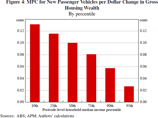
Critically, these estimated average MPCs mask substantial heterogeneity by household income. Regressions (5) and (6) augment regressions (1) and (2) with an interaction between the dollar change in gross housing wealth and household median income. The interaction term is negative, and statistically significant, indicating that low-income households are more likely to purchase a new vehicle out of a dollar change in gross housing wealth than high-income households. Using the regression estimates, Figure 4 graphs the estimated MPC for different levels of postcode-level household median income, assuming the same purchase price for vehicles across postcodes. The estimated MPC for new vehicles per dollar change in gross housing wealth is 0.12 cents for a postcode at the 25th percentile of income, 0.10 cents at the 50th percentile, and 0.03 cents at the 95th percentile. Using postcode-level mean rather than median household income gives similar estimates (see regressions (1) and (2) in Table A1). As a caveat, note that the lower propensity of high-income households to purchase a new vehicle out of an increase in housing wealth could be partly offset by high-income households purchasing relatively expensive vehicles. Unfortunately, we do not have data on average new vehicle purchase price by postcode. However, differences in average purchase prices would have to be large to offset the large differences in propensity to purchase a new vehicle out of housing wealth.
Heterogeneity in MPCs means that the aggregate MPC is different to an unweighted average of MPCs across households. A given economy-wide percentage change in house prices results in much larger dollar changes in housing wealth for high- than low-income households, because high-income households tend to own higher-valued homes.[15] Despite this, high-income households contribute relatively little to aggregate consumption growth because they have a low MPC out of housing. Below-median income households have a high MPC, but own a relatively small share of the housing stock by value, and so make a smaller contribution to aggregate consumption growth than their numbers would suggest.
Much of the existing literature has emphasised heterogeneity in MPCs by household age, rather than income (e.g. Browning et al 2013; Windsor et al (2013). The heterogeneity in MPC by income that we identify is not a result of age being an omitted variable. While there is a strong correlation between age and income at the household level, at the postcode level – our unit of observation – the correlation between average age and median income is low. Including categorical age dummies as additional explanatory variables has a small effect on the estimated heterogeneity in MPC by income class (see regressions (3) and (4) in Table A1).[16]
Footnotes
This calculation uses data from the 2009–10 ABS Household Expenditure Survey and the 2009–10 ABS Household Wealth and Wealth Distribution data. The elasticity of new vehicle consumption with respect to gross housing wealth is assumed to be 0.45, around the midpoint of our estimates in Table 3, and vehicle consumption is assumed to be 2.9 per cent of total consumption, its average since 2000 based on national accounts data. The price of new vehicles is assumed to be unaffected by changes in house prices. [12]
The average price of a new passenger vehicle can be estimated by dividing household final consumption expenditure – purchase of vehicles in the national accounts by the total number of sales to private buyers, sourced from VFACTS. These data indicate an average new passenger vehicle price of $38,900 in 2006 and $33,200 in 2011. The use of national accounts data to estimate an average vehicle price is problematic because the consumption measure includes dealer margins on sales of used vehicles to households, upwardly biasing our estimate. We view the change in average price between 2006 and 2011 to also be implausibly large. The CPI motor vehicles price index indicates only a 4.4 per cent decline over the same period, part of which represents estimated quality change rather than lower retail prices. To estimate a lower-bound on the average price of a new passenger vehicle, we take a sales-weighted average of prices for the top-selling passenger vehicles in 2014, using the base model list price for each vehicle type. This gives an average price of about $24,300. In the absence of alternative data we assume, somewhat arbitrarily, an average price for new passenger vehicles of $30,000 in both 2006 and 2011 – roughly the midpoint of the different estimates. If our estimate is too small, our MPC estimates should be scaled up proportionately, and vice versa. [13]
It is perhaps surprising that the estimated MPC for new passenger vehicles out of a dollar change in postcode-level income is not close to unity. Individual-level transitory income shocks should cancel out at the postcode level, revealing an almost one-to-one relationship between consumption and income. Two factors likely account for the small estimated MPC out of income. Firstly, we have included a range of control variables correlated with income, such as the unemployment rate. Secondly, while measurement error in incomes is likely to be small relative to the level of income, it is likely to be large relative to changes in incomes over a five-year period, attenuating the coefficient on the income variable. Some measurement error arises because the Census collects income data as a categorical rather than a continuous variable. [14]
The positive association between income and house value and the estimated decline in MPC with income together imply that the MPC is highest in postcodes with low average house value. A direct way to see this is to replace the income interaction term for regressions (5) and (6) in Table 6 with an interaction between the dollar change in housing equity and the level of house prices. Regressions (5) and (6) in Table A1 show that this term is negative, and statistically significant. [15]
The MPC for middle-age (41–55 years of age) households is estimated to be a little larger than for young (23–40 years of age) and old households (55 and over), but the lack of variation in average age across postcodes means that the effect is imprecisely estimated. [16]