RDP 2014-04: Home Price Beliefs in Australia 5. Measuring Home Valuation Differences
May 2014 – ISSN 1320-7229 (Print), ISSN 1448-5109 (Online)
- Download the Paper 801KB
5.1 Distribution of Home Valuation Differences
Using home valuation differences to make inferences about household belief formation is the focus of this paper. As discussed in the previous section, we could construct these valuation differences by comparing the (unconditional) average sale price to the average self-assessed home value within each postcode and time period. This comparison is given by Equation (3):
However, this measure confounds a comparison of ‘true’ prices with changes in the composition of homes sold or self-assessed each period. For example, if the homeowners that drop out of the HILDA Survey over time are more likely to own smaller homes, then the size of homes self-assessed each year in the HILDA Survey will be increasing (attrition due to refusal, death or inability to locate the respondent is an issue in all panel surveys). Accordingly, for each postcode the change in average self-assessed home values each year will reflect ‘true’ price changes as well as the change in the composition of homes. This would, in turn, lead to valuation differences that are artificially inflated, with the bias increasing over time.
Compositionally adjusted estimates can be constructed by comparing the postcode-time dummy coefficients from Equation (1) and Equation (2):
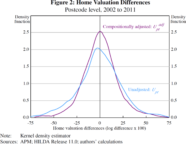
The density of Upt versus  is plotted in Figure 2. In comparing these
densities, two characteristics can be observed. First, both densities appear
centered around zero. Second, the density of home valuation differences is
less dispersed on a compositionally adjusted basis than on a raw basis with
a standard deviation of 20 per cent versus 26 per cent.

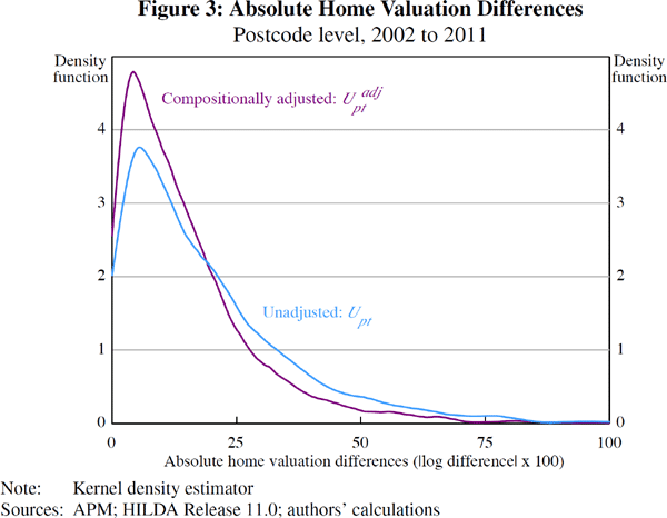
The density of the absolute value of the home valuation differences is shown in Figure 3. On a compositionally adjusted basis, half of all postcodes provide an average valuation within 11 per cent of the average market value and three-quarters provide a valuation within 20 per cent.

The characteristics of home valuation differences ( )
are summarised in Table 1. On average, across all cities, the differences have
a mean that is positive at 0.5 per cent, but this is not statistically different
to zero. This suggests that the average homeowner is unbiased in their subjective
home valuation. However, this aggregate picture masks some small biases in
different capital cities. In Sydney, for instance, home valuation differences
are significantly positive on average, at around 1.8 per cent. Likewise in
Brisbane, there is a significantly positive home valuation difference of 2.8
per cent. But, in Melbourne there is a negative home valuation difference of
around 2.2 per cent, on average.
| All cities | Sydney | Melbourne | Brisbane | |
|---|---|---|---|---|
| Moments | ||||
| Mean (%) | 0.5 | 1.8*** | −2.2*** | 2.8*** |
| 95% confidence interval | (−0.3 to 1.3) | (0.6 to 3.1) | (−3.3 to −1.1) | (0.7 to 4.9) |
| Standard deviation (%) | 20.3*** | 19.7*** | 17.8*** | 24.9*** |
| 95% confidence interval | (19.4 to 21.3) | (18.6 to 20.8) | (16.5 to 19.0) | (22.1 to 27.7) |
| Skewness | −0.2 | 0.3** | −0.1 | −0.8** |
| 95% confidence interval | (−0.6 to 0.2) | (0 to 0.5) | (−0.7 to 0.5) | (−1.6 to −0.0) |
|
Notes: Confidence intervals calculated via a bootstrap; ***, ** and * indicate significance at the 1, 5 and 10 per cent level, respectively Sources: APM; HILDA Release 11.0; authors' calculations |
||||
5.2 Significance of Home Valuation Differences
We now examine whether the differences between self-assessed values and sale prices across different postcodes are statistically significant. To determine the statistical significance of the postcode differences it is helpful to nest Equations (1) and (2):
where Pdpt is the price of home d in postcode p in time period t (both self-assessed and sold) and where the dummy variable Sdpt takes the value of 1 if the observed price is self-assessed and a value of 0 if the observed price is a sale price. All other notation is as defined previously. Equation (5) is estimated separately for each city, with the κpt coefficients providing an estimate of the home valuation difference for each postcode and time period.
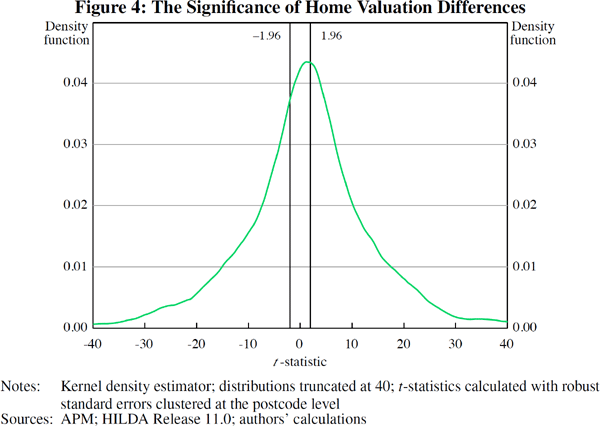
Our main interest is in the significance of the κpt coefficients, which allow us to make inferences about the mass of statistically significant valuation differences. To this end, in Figure 4 we plot the t-statistics for each home valuation difference κpt estimated in Equation (5) in each postcode and time period.

We find that about four-fifths of the home valuation differences are statistically significant at conventional levels. This suggests that our finding of no bias on average partly reflects offsetting, significant, differences. In other words, there is a distribution of valuation differences across postcodes; at any point in time, some postcodes have self-assessed valuations that appear high relative to market-inferred prices while some postcodes have valuations that appear low relative to market-inferred prices, on average.


