RDP 2014-04: Home Price Beliefs in Australia 4. Hedonic Methodology

A simple metric for measuring home valuation differences would be to compare, at a given point in time, the average self-assessed home value of each surveyed homeowner within a postcode (from the HILDA Survey) to the average price of all homes sold in that postcode (from the APM dataset). For example, using the available data for Sydney and quarterly time periods over the period 2002 to 2011, we would obtain 5,840 (= 40 quarters × 146 postcodes) price comparisons; the mean of which would measure the overall home valuation difference. However, at any point in time there could be systematic differences in the composition of properties self-assessed and sold within postcodes, thereby complicating this simple comparison.

To account for this, we use hedonic regression methods, which are common in the home-price measurement literature. The hedonic adjustment method determines, for each postcode and time period, the mean price of homes sold (or self-assessed) conditional on the characteristics of homes sold (or self-assessed). These ‘conditional mean’ estimates are designed to capture the level of home prices, holding constant any compositional changes in the homes sold or self-assessed each period. Therefore, the estimates measure the change in home values solely due to the passage of time.

We use postcode-time dummy hedonic models. The hedonic models for the sale price of homes and self-assessed home values are given by Equation (1) and Equation (2) respectively.^[7]

In Equation (1), S_ipt denotes the sale price of each home i in postcode p in quarter t. In Equation (2), V_jpt denotes the value of a self-assessed home j in postcode p in quarter t.

A home's characteristic is denoted by y_c for c = 1,2,…C. These characteristics are common across the sale and valuation equations and include dummy variables for the number of bedrooms and housing type (i.e. house or unit). The coefficient β_c captures the value of a given characteristic.^[8]

The dummy variable, D_ipt , takes the value of 1 if the home sold or self-assessed is from postcode-time pt, and 0 otherwise. Our interest is in the coefficients on the postcode-time fixed effects for the log of sale prices and the log of self-assessed home values . In a given time period, these measure the average value of homes sold or self-assessed within a postcode, after controlling for the characteristics of homes sold or self-assessed.

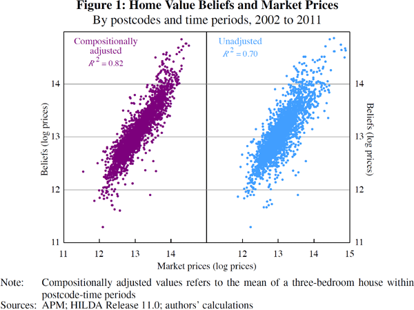
The effect of hedonic (or composition) adjustments on sale prices and self-assessed home values is shown in Figure 1 (regression output is shown in Table A1). The compositionally adjusted scatter plot (left panel) shows the association between average sale prices from Equation (1) and average self-assessed home values from Equation (2) across postcodes. An unadjusted comparison is presented in the right panel, and shows the association between unconditional mean sale prices, , and self-assessed home values, , across postcodes.

The correlation between adjusted prices is stronger than the correlation between unadjusted prices (0.91 versus 0.84). This suggests compositionally adjusting the data is important when estimating the difference between average home valuations and sales prices across postcodes.

Footnotes

Following Hansen (2009), each capital city is treated as a separate market with the hedonic models estimated separately for Sydney, Melbourne and Brisbane. [7]

In order to match the hedonic model that could be estimated for self-assessed home values using the HILDA dataset, a number of relevant housing characteristics – available in the APM dataset – have been excluded from Equation (1). These include the number of bathrooms, parking spaces and sale mechanism (i.e. auction or private treaty). Therefore, estimates of the value of a bedroom and the value of a postcode may be biased if these variables are correlated with any omitted characteristics in Equations (1) and (2). The robustness of our results to this potential source of bias is examined in detail in Section 8. [8]