RDP 2010-07: Monetary Policy and the Exchange Rate: Evaluation of VAR Models 4. VAR Models with Simulated Data
September 2010
- Download the Paper 335KB
In this section, we estimate a selection of VAR models using simulated data from
the DSGE model. As our baseline experiment, we simulate 500 observations from
the DSGE model for the following variables (using the posterior mean of the
estimated parameters in Table 1):  (foreign output);
  (foreign inflation);
  (foreign interest rate);
yt (domestic output); πt (domestic
inflation); rt (domestic interest rate); and qt
(the real exchange rate). These variables are the ones that researchers typically
use to estimate VAR models. Consistent with the small open economy assumption,
we impose block exogeneity, with foreign variables unaffected by domestic shocks.
We estimate VARs of order two, consistent with the VAR representation of the
DSGE model.
The size of the monetary policy shock is normalised to 25 basis points. This ensures that the differences between the true IRF's and the estimated IRF's are not simply due to a bias in estimating the size of the policy shock. Since we generate large amounts of data (500 observations), no confidence intervals are presented with the subsequent figures.
4.1 Recursive VARs
Using our simulated data, we estimate a recursive VAR based on the ordering given
above – that is,  ,
,
 ,
,
 ,
yt, πt, rt and
qt – with the real exchange rate being the most endogenous
variable (that is, it responds contemporaneously to all of the other variables).
We call this Ordering (1). Some studies identify monetary policy by restricting
the exchange rate from reacting immediately to a monetary policy shock (see
Mojon and Peersman 2001; Peersman and Smets 2003). Thus, we also swap the ordering
of the last two variables to make the domestic interest rate the most endogenous
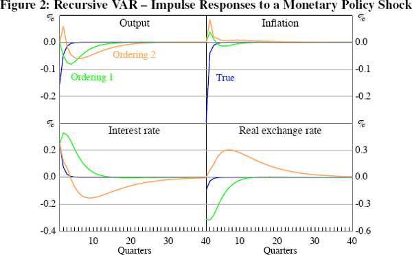
variable (we call this Ordering (2)). Figure 2 compares the impulse responses
from the recursive models with the true responses from the DSGE model. Similar
to Carlstrom, Fuerst and Paustian (2009), the magnitudes and shapes of the
impulse responses are at odds with the results from the DSGE
model.[7]
Ordering (2) exhibits the exchange rate puzzle, with the exchange rate depreciating
following the contraction in monetary policy; moreover, output rises at first
in response to the monetary policy contraction. Ordering (1) produces a real
exchange rate appreciation, but the size of the appreciation is much larger
than the theoretical response. In the DSGE model, monetary policy and the exchange
rate interact contemporaneously, so it seems likely that the puzzles relating
to the real exchange rate follow from the ‘zero-type’ restrictions
which prevent this (see also Faust and Rogers 2003; Bjørnland and Halvorsen
2008). Both VAR models produce the price puzzle, with inflation rising following
the monetary policy shock. Figure 2 highlights the fact that the estimates
of the impulse responses are sensitive to identifying assumptions (that is,
Orderings (1) and (2) are quite different). Overall, the results suggest that
care should be taken when using VAR models of this type to identify the monetary
transmission mechanism.
4.2 Sign-restricted VARs
We now examine how well sign-restricted VARs can identify monetary policy shocks. These models achieve identification by imposing the direction that key variables will move (over a given horizon) in response to different types of shocks. Full details of the sign-restricted VAR methodology are provided in Appendix A.
The set of sign restrictions adopted in the paper is presented in Table 2. Given that the foreign variables enter the DSGE model as exogenous processes, we assume that domestic shocks do not affect the foreign variables, while the response of the domestic variables to the foreign shocks are left unrestricted. We also remain agnostic about the response of the exchange rate to all of the shocks in the model. In particular, we leave the response of the real exchange rate to a domestic monetary policy shock unrestricted because we want to see whether the sign restrictions on other variables are sufficient to identifying impulse responses, which are free of exchange rate puzzles. We avoid price and output puzzles by assuming that inflation and output fall in response to a contractionary monetary policy shock. The sign restrictions are imposed for the impact quarter only.[8] In contrast, Paustian (2007) and Scholl and Uhlig (2008) allow the restrictions to be imposed for a longer period of time. We return to this issue in Section 4.3.
| Shock to: | y* | π* | r* | y | π | r | q |
|---|---|---|---|---|---|---|---|
| Foreign demand | ↑ | ↑ | ↑ | – | – | – | – |
| Foreign productivity | ↑ | ↓ | ↓ | – | – | – | – |
| Foreign monetary policy | ↓ | ↓ | ↑ | – | – | – | – |
| Demand | 0 | 0 | 0 | ↑ | ↑ | ↑ | – |
| Productivity | 0 | 0 | 0 | ↑ | ↓ | ↓ | – |
| Monetary policy | 0 | 0 | 0 | ↓ | ↓ | ↑ | – |
| Notes: ↑ (↓) means positive (negative) response of the variables in columns to shocks in rows. 0 means no response (as implied by the small open economy assumption). – means no restriction is imposed on the response. | |||||||
Figure 3 compares the responses of the variables to a monetary policy shock under the sign-restricted VAR model with those from the true model (the dark blue line). The shaded area represents the area between the 5th and 95th percentiles of the responses generated from the sign-restricted VAR algorithm, and the red line plots the median of the set of identified responses. Fry and Pagan (forthcoming) have criticised the practise of using the median of the distribution of responses as a location measure, since the median at each horizon and for each variable may be obtained from different candidate models. They suggest using a single unique draw that is closest to the median impulse responses for all variables. Accordingly, the pink line plots this so-called ‘median target’ (MT) measure.[9] The same criticism applies to any other percentile measure such as the shaded area presented here. We also show a unique draw that minimises the distance from the true impulses (shown by the light blue line and labelled as the ‘true target’ (TT)).
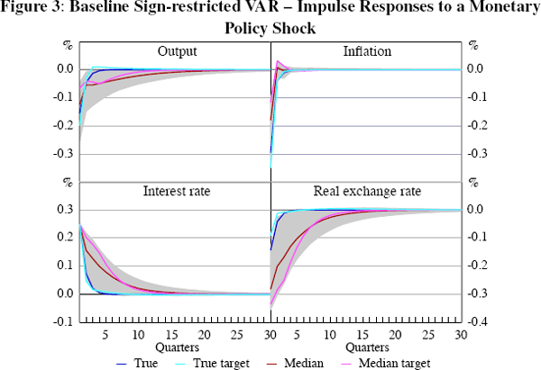
As shown in Figure 3, the sign-restricted VAR does a significantly better job than the recursive VAR models at replicating the true impulse responses to a contractionary monetary policy shock. The model captures correctly the sign of the real exchange rate response on impact. However, the range of responses (shown by the shaded area) is quite wide, even for those variables whose response is constrained a priori.[10],[11] Responses characterising the central tendency of the sign-restricted VAR (the median and MT measures) are more persistent than those of the DSGE model. This may be because the VAR model is only partially identified by the set of restrictions shown in Table 2. There may be unidentified shocks which happen to satisfy the sign restrictions placed on the monetary policy shock, or indeed any of the other shocks we are attempting to identify. In other words, these unidentified shocks contaminate the central tendency measures that utilise all accepted draws.[12]
These results suggest that the median does not necessarily capture the true model, as it is often thought to do. For instance, on impact the true responses of output, inflation and the real exchange rate to the monetary policy shock are located on the 36th, 9th and 94th percentiles, respectively; nowhere near the 50th percentile – the median. The unique draw closest to the true impulse responses (the TT measure) is better than the central tendency measures by construction, but there are still some small discrepancies. Moreover, the biases are even more prominent for the identified demand and productivity shocks (see Figures C1 and C2), probably due to the presence of the unidentified shock in the sign-restricted VAR model.
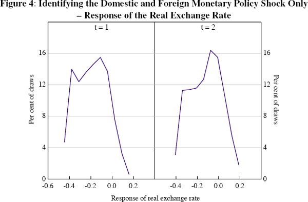
It is likely that the number of identified shocks and identification restrictions employed matters for the performance of the sign-restricted VAR model. The results above are based on identifying six shocks with restrictions on six of the variables. If instead, we only identify the monetary policy shocks (both foreign and domestic), the exchange rate puzzle re-emerges. The results are summarised in Figure 4, which shows histograms of the response of the real exchange to an unexpected tightening of monetary policy on impact (the left panel in the figure) and one period after (the right panel). It can be seen that around 10 and 24 per cent of the 1,000 draws imply a depreciation of the real exchange rate on impact and one quarter after the shock, respectively. In addition, uncertainty surrounding the responses of all other variables increases slightly. This suggests that the identified monetary policy shock is contaminated with features of other structural shocks that are left unidentified (the ‘multiple shocks problem’), and as a result the ‘agnostic’ sign restriction approach of Scholl and Uhlig (2008) may not be able to recover ‘true’ impulse responses. In short, it appears that the likelihood of recovering the correct sign of the exchange rate increases with the number of identified shocks.
4.3 Extensions
In addition to the presence of unidentified shocks, there are other reasons why there may be biases inherent in the sign-restricted VAR results which are worth examining. These include: the number of sign restriction periods; the number of lags in the VAR model; and the relative strength of the ‘true’ shock signal.
It has been argued that a longer horizon over which the sign restrictions are enforced may be required in order to better match the theoretical responses. According to Paustian (2007), however, as the horizon for the sign restrictions is extended, the distribution of the responses actually becomes centred further away from the true impact responses. This is likely with our simulated data as well, given the instantaneous response of the model variables to the shocks; although imposing sign restrictions over two quarters yields broadly unchanged impulse responses.
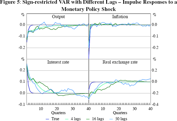
Given that we use only a subset of model variables in the VAR, we may be introducing truncation bias by estimating a finite order VAR model. Kapetanios, Pagan and Scott (2007) investigate this question in a simulation exercise. They find that 50 lags were required to produce estimated impulse responses that are essentially indistinguishable from the true values.[13] If increasing the lag length were to improve the model fit in our experiment, it is plausible that the number of draws required to yield a model which satisfies the identifying restrictions should decline with the lag length. However, this turns out not to be the case. Table 3 shows the average number of draws required to find a decomposition that satisfies the sign restrictions given in Table 2 for different lag length specifications. As the lag length increases, the number of draws initially decreases, but the sign restriction algorithm requires a greater number of draws to find a satisfactory draw when the lag length is increased beyond 16. Figure 5 shows the impulses responses with different lag lengths. There is very little, if any, evidence that increasing the lag length improves the accuracy of the estimated impulse responses.
| Lag length | L = 1 | L = 2 | L = 4 | L = 8 | L = 16 | L = 32 | L = 50 |
|---|---|---|---|---|---|---|---|
| Total/Accepted | 40.023 | 39.483 | 39.106 | 38.94 | 36.2810 | 40.367 | 42.021 |
| Note: Total/Accepted indicate the average number of draws required to find a decomposition that satisfies the sign restrictions given in Table 2. | |||||||
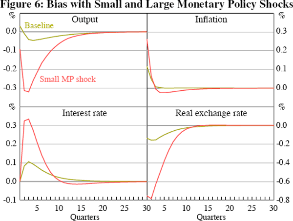
It is possible that if the variance of the monetary policy shock is small it may be difficult for the VAR model to properly identify monetary policy innovations. Faust and Rogers (2003) are unable to find policy shocks that generate interest rate and exchange rate responses consistent with UIP, and conclude that US monetary policy shocks may explain less of the observed exchange rate variability than previously believed. Paustian (2007) also reviews this possibility, and concludes that the variance of the shock under study must be sufficiently large in order to deliver the correct sign of the unconstrained impulse response. However, we can show that our modelling does not suffer this particular problem. Even if the standard deviation of the monetary policy shock (σr) in the underlying DSGE model is reduced (we tested lowering σr 1,000 fold), the sign of the real exchange rate response is correctly identified using our sign-restricted VAR. Although, as shown in Figure 6, decreasing the variance of the monetary policy shock increases estimation biases (measured as the deviation from the ‘true’ impulse response).
Footnotes
Carlstrom et al simulate data from a three-equation DSGE model that is consistent with the timing assumptions of the standard Choleski identification. They assume that output and prices in the theoretical model are determined before the realisation of the monetary policy shock. Consequently, inflation and the output gap do not respond contemporaneously to the monetary shock. They still find that there are large differences between the true IRFs and the estimated IRFs. [7]
It is worth emphasising that we impose strict exogeneity of the foreign variables, that is, the feedback from the domestic variables on the foreign variables is always zero, not just on the impact period. [8]
Though we focus here on the monetary policy shock, this measure finds a unique draw that minimises the distance from the medians for all identified shocks. [9]
As a cross-check, we also restrict the real exchange rate to appreciate on impact following a contractionary monetary policy shock. This has little effect on the range of responses of domestic output, inflation and the interest rate. [10]
It has been argued that in order to reduce the dispersion in the set of models, that is, the width of the band, additional quantitative information about the likely magnitude (or the shape) of the impulse responses might be required (Uhlig 2005; Kilian and Murray 2010; Fry and Pagan forthcoming). [11]
There are seven variables in the model but we only identify six shocks. Hence, there is one unidentified shock on which we impose no sign restrictions. Fry and Pagan (forthcoming) note that this can lead to the multiple shocks problem, in which unidentified shocks can be similar to shocks which have been identified using sign restrictions. [12]
Their empirical model suffers from the missing variables problem. There are 26 variables in their theoretical model but only 6 in the empirical one. [13]