RDP 2010-07: Monetary Policy and the Exchange Rate: Evaluation of VAR Models Appendix A: Sign Restriction Algorithm

Consider a general VAR(p) model with n variables Y_t:

where: A(L) = A₁L + ... + A_pL^p is a p^th order matrix polynomial; B is a (n × n) matrix of coefficients that reflect the contemporaneous relationships among Y_t; and ε_t is a set of (n × 1) normally distributed structural disturbances with mean zero and variance covariance matrix Σ, Σ_i,j = 0∀i ≠ j. The structural representation has the following reduced form:

where π(L) = B⁻¹A(L) and e_t is a set of (n × 1) normally distributed reduced-form errors with mean zero and variance covariance matrix V, V_i,j ≠ 0∀i,j. The aim is to map the statistical relationships summarised by the reduced-form errors e_t back into economic relationships described by ε_t. Let P = B⁻¹. The reduced-form errors are related to the structural disturbances in the following manner:

for some matrix H such that HH^′ = p∑p^′. An identification problem arises if there are not enough restrictions to uniquely pin down H from the matrix V.

The central idea behind SVAR analysis is to decompose the set of reduced-form shocks, characterised by V, into a set of orthogonal structural disturbances characterised by ∑. However, there are an infinite number of ways in which this orthogonality condition can be achieved. Let H be an orthogonal decomposition of V = HH′. The multiplicity arises from the fact that for any orthonormal matrix Q (where QQ′ = I), such that is also an admissible decomposition of V, where . This decomposition produces a new set of uncorrelated shocks , without imposing zero-type restrictions on the model.

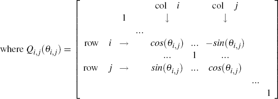
Define an (n × n) orthonormal rotation matrix Q such that:

where θ_i,j ∈ [0, π]. This provides a way of systematically exploring the space of all VMA representations by searching over the range of values θ_i,j. We generate the Qs randomly from a uniform distribution using the following algorithm:

1. Estimate the VAR to obtain the reduced form variance covariance matrix V.
2. For both the foreign and domestic block, draw a vector θ_i,j from a uniform [0, π] distribution.
3. Calculate Q, as in Equation (A4).
4. Use the candidate rotation matrix Q to compute ε_t = HQe_t and its corresponding structural IRFs for domestic and foreign shocks.
5. Check whether the IRFs satisfy all the sign restrictions described in Table 2. If so, keep the draw, if not, drop the draw.
6. Repeat (2)–(5) until 1,000 draws that satisfy the restrictions are found.