RDP 2008-07: A Medium-scale Open Economy Model of Australia 4. Empirical Results
December 2008
- Download the Paper 485KB
This section reports the results of the estimation exercise.
4.1 The Benchmark Specification
In the benchmark estimation of the model we use the inflation-targeting sample, that is, data from 1993:Q2 to 2007:Q3. We estimate a total of 56 parameters compared to the 51 parameters estimated by Adolfson et al (2007). While Adolfson et al calibrate the elasticity of consumption goods to changes in the relative price of imported and domestically produced goods (ηc), and the persistence of the medium-run inflation target (ρπ) and wage mark-up (λw), we estimate these parameters. We also estimate the persistence and innovation variance of the commodity demand and price shocks that are absent in Adolfson et al.
Tables 1 and 2 report the statistics of the prior and estimated posterior distributions of the structural parameters. In Appendix D the same information is given in Figures D1–D4, where we plot the estimated posterior distributions of the model's parameters together with their prior distributions as well as their constant weight prior estimates.
| Parameter Distribution | Prior | Posterior | ||||||
|---|---|---|---|---|---|---|---|---|
| Mode | Std | Mean | Std | 5% | 95% | |||
| Price stickiness | ||||||||
| ξw | beta | 0.675 | 0.050 | 0.629 | 0.048 | 0.550 | 0.706 | |
| ξd | beta | 0.675 | 0.010 | 0.688 | 0.009 | 0.673 | 0.704 | |
| ξm,c | beta | 0.675 | 0.010 | 0.674 | 0.010 | 0.658 | 0.691 | |
| ξm,i | beta | 0.675 | 0.010 | 0.674 | 0.010 | 0.657 | 0.690 | |
| ξx | beta | 0.675 | 0.010 | 0.678 | 0.053 | 0.588 | 0.761 | |
| ξe | beta | 0.675 | 0.050 | 0.620 | 0.038 | 0.555 | 0.677 | |
| Indexation | ||||||||
| κw | trunc uniform | [0,1] | 0.552 | 0.229 | 0.145 | 0.906 | ||
| κd | trunc uniform | [0,1] | 0.890 | 0.091 | 0.714 | 0.992 | ||
| κm,c | trunc uniform | [0,1] | 0.347 | 0.226 | 0.037 | 0.783 | ||
| κm,i | trunc uniform | [0,1] | 0.083 | 0.081 | 0.004 | 0.247 | ||
| κx | trunc uniform | [0,1] | 0.089 | 0.087 | 0.005 | 0.258 | ||
| Mark-ups | ||||||||
| λd | Inv gamma | 1.200 | 2.000 | 10.60 | 4.456 | 5.461 | 19.63 | |
| λm,c | Inv gamma | 1.200 | 2.000 | 2.129 | 0.740 | 1.229 | 3.597 | |
| λm,i | Inv gamma | 1.200 | 2.000 | 3.437 | 0.983 | 2.154 | 5.358 | |
| Investment friction and habits | ||||||||
 |
normal | 7.694 | 2.500 | 5.709 | 1.801 | 3.048 | 8.973 | |
| b | beta | 0.650 | 0.100 | 0.760 | 0.051 | 0.673 | 0.843 | |
| Substitutions of elasticity | ||||||||
| ηc | trunc uniform | [1,∞) | 1.301 | 0.286 | 1.016 | 1.911 | ||
| ηi | trunc uniform | [1,∞) | 1.462 | 0.318 | 1.078 | 2.076 | ||
| ηf | trunc uniform | [1,∞) | 1.129 | 0.123 | 1.007 | 1.378 | ||
| Risk premium | ||||||||
 |
inv gamma | 0.010 | 0.001 | 0.001 | 0.001 | 0.000 | 0.002 | |
| Technology growth | ||||||||
| μz | trunc uniform | 1.008 | 0.001 | 1.009 | 0.000 | 1.009 | 1.009 | |
| Monetary policy | ||||||||
| ρR | beta | 0.800 | 0.050 | 0.836 | 0.025 | 0.793 | 0.874 | |
| rπ | normal | 1.750 | 0.100 | 1.750 | 0.097 | 1.587 | 1.909 | |
| rΔπ | normal | 0.000 | 0.100 | 0.090 | 0.066 | −0.018 | 0.198 | |
| rx | normal | 0.010 | 0.005 | −0.009 | 0.004 | −0.016 | −0.003 | |
| ry | normal | 0.125 | 0.100 | −0.024 | 0.011 | −0.043 | −0.009 | |
| rΔy | normal | 0.000 | 0.100 | 0.035 | 0.020 | 0.004 | 0.068 | |
| Parameter Distribution | Prior | Posterior | ||||||
|---|---|---|---|---|---|---|---|---|
| Mode | Std | Mean | Std | 5% | 95% | |||
| Exogenous processes – AR(1) coefficients | ||||||||
 |
beta | 0.500 | 0.275 | 0.946 | 0.021 | 0.906 | 0.970 | |
| ρε | beta | 0.500 | 0.150 | 0.593 | 0.074 | 0.467 | 0.713 | |
| ρϒ | beta | 0.500 | 0.150 | 0.426 | 0.084 | 0.291 | 0.565 | |
 |
beta | 0.500 | 0.275 | 0.550 | 0.278 | 0.083 | 0.957 | |
 |
beta | 0.500 | 0.275 | 0.970 | 0.029 | 0.912 | 0.996 | |
 |
beta | 0.500 | 0.275 | 0.076 | 0.060 | 0.007 | 0.196 | |
 |
beta | 0.500 | 0.100 | 0.485 | 0.100 | 0.323 | 0.654 | |
 |
beta | 0.500 | 0.275 | 0.999 | 0.000 | 0.998 | 0.999 | |
 |
beta | 0.500 | 0.275 | 0.092 | 0.084 | 0.007 | 0.261 | |
 |
beta | 0.500 | 0.275 | 0.093 | 0.085 | 0.007 | 0.261 | |
 |
beta | 0.500 | 0.275 | 0.608 | 0.123 | 0.380 | 0.797 | |
| ρpcom | beta | 0.500 | 0.275 | 0.965 | 0.023 | 0.923 | 0.992 | |
| ρcom | beta | 0.500 | 0.275 | 0.998 | 0.001 | 0.996 | 0.999 | |
| Exogenous processes – standard deviations (×10−2) | ||||||||
 |
trunc uniform | [0,∞) | 0.127 | 0.029 | 0.084 | 0.180 | ||
| σε | trunc uniform | [0,∞) | 1.228 | 0.197 | 0.929 | 1.573 | ||
| σϒ | trunc uniform | [0,∞) | 0.954 | 0.167 | 0.701 | 1.249 | ||
 |
trunc uniform | [0,∞) | 0.054 | 0.039 | 0.005 | 0.130 | ||
 |
trunc uniform | [0,∞) | 0.090 | 0.024 | 0.056 | 0.134 | ||
 |
trunc uniform | [0,∞) | 0.402 | 0.051 | 0.323 | 0.489 | ||
 |
trunc uniform | [0,∞) | 0.402 | 0.303 | 0.033 | 0.974 | ||
 |
trunc uniform | [0,∞) | 0.144 | 0.030 | 0.097 | 0.194 | ||
 |
trunc uniform | [0,∞) | 0.360 | 0.103 | 0.216 | 0.551 | ||
 |
trunc uniform | [0,∞) | 3.870 | 0.995 | 2.325 | 5.621 | ||
 |
trunc uniform | [0,∞) | 5.178 | 1.002 | 3.639 | 6.956 | ||
| σr | trunc uniform | [0,∞) | 0.022 | 0.016 | 0.002 | 0.053 | ||
 |
trunc uniform | [0,∞) | 0.554 | 0.136 | 0.358 | 0.780 | ||
| σcom | trunc uniform | [0,∞) | 2.368 | 0.247 | 2.003 | 2.809 | ||
| σpcom | trunc uniform | [0,∞) | 4.895 | 0.773 | 3.743 | 6.627 | ||
The parameters appear to be for the most part tightly estimated given that posterior standard deviations are smaller than the prior standard deviations. It seems, however, that the data are not very informative regarding the degree of price stickiness in the imported consumption, imported investment and export sectors (ξm,c, ξm,i and ξx) since the posterior distributions do not differ a lot from their prior distributions. The constant weight prior posterior distributions of the ξ parameters provide further evidence of parameter under-identification: the posterior distributions tend to be rather flat. In a situation like this, the prior plays a crucial role in making inferences. The priors (and estimated parameter values) imply that prices are re-optimised at least around every three quarters.[6]
Data seem more informative on the indexation parameters (κw, κd, κm,c, κm,i and κx), which vary significantly across the different sectors of the economy. (As a cross-check we imposed informative priors on these parameters, centred around 0.5, and obtained similar posterior distributions as shown in Figure D1, albeit slightly less dispersed.) The indexation parameters on imported investment goods (κm,i) and exports (κx) are quite low, suggesting that these Phillips curves are mostly forward-looking. The indexation parameters for the domestic good (κd), the imported consumption good (κm,c) and the wage (κw) imply more persistence. The habit formation parameter (b) has a posterior mean of 0.76, reflecting a large degree of inertia in consumption. The value of the elasticity of substitution between home and foreign consumption goods (ηc) is only 1.30, much lower than the calibrated value in Adolfson et al (2007). This could reflect relatively high estimates of steady-state price mark-ups (λd, λm,c, λm,i). It is worth noting, however, that when we calibrated the mark-up parameters at the prior modes, this raised the estimate of ηc but did not produce drastically lower marginal likelihoods.
The parameters of the policy reaction function are well identified. There are some differences between the Bayesian and constant weight prior posteriors, due to the informative priors imposed on the policy parameters. The constant weight prior estimate of the inflation response in the policy rule implies a stronger reaction of interest rates to inflation movements in comparison with the Bayesian estimate.
Although we allow for both temporary and permanent productivity shocks, the estimated persistence of some of the transitory shocks is quite large. The posterior distributions of the AR parameters of the consumption preference (ρζc), imported consumption mark-up (ρλm,c) and commodity price (ρλpcom) shocks all have a lot of mass around 1.
The standard deviation of the innovations to the temporary productivity shock (σe) is smaller than that of the permanent productivity shock (σμz). Shocks for imported investment and export mark-ups, consumption preferences, commodity demand and commodity prices are the most volatile in the estimated model.
4.2 The Dynamics of the Estimated Model
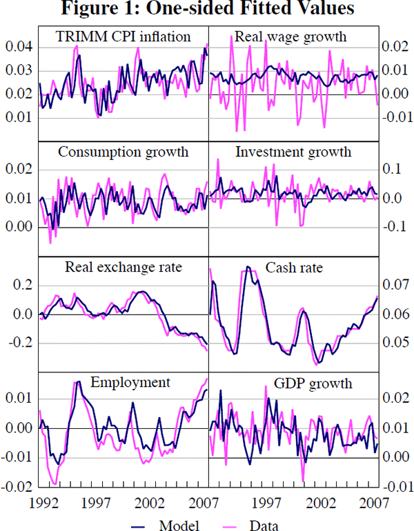
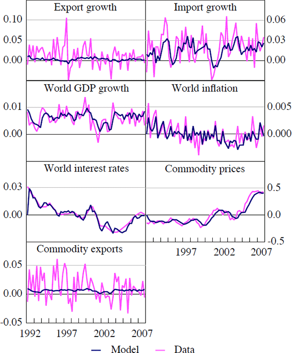
Figure 1 shows the one-sided fit of the model. The fit for most of the variables is good; the exceptions are real wage, export and commodity export growth.[7] These variables are quite volatile at a quarterly frequency, and hard to predict, so the failure of fitting these series is not necessarily a weakness of the model as the best predictor for a white noise process is its mean.


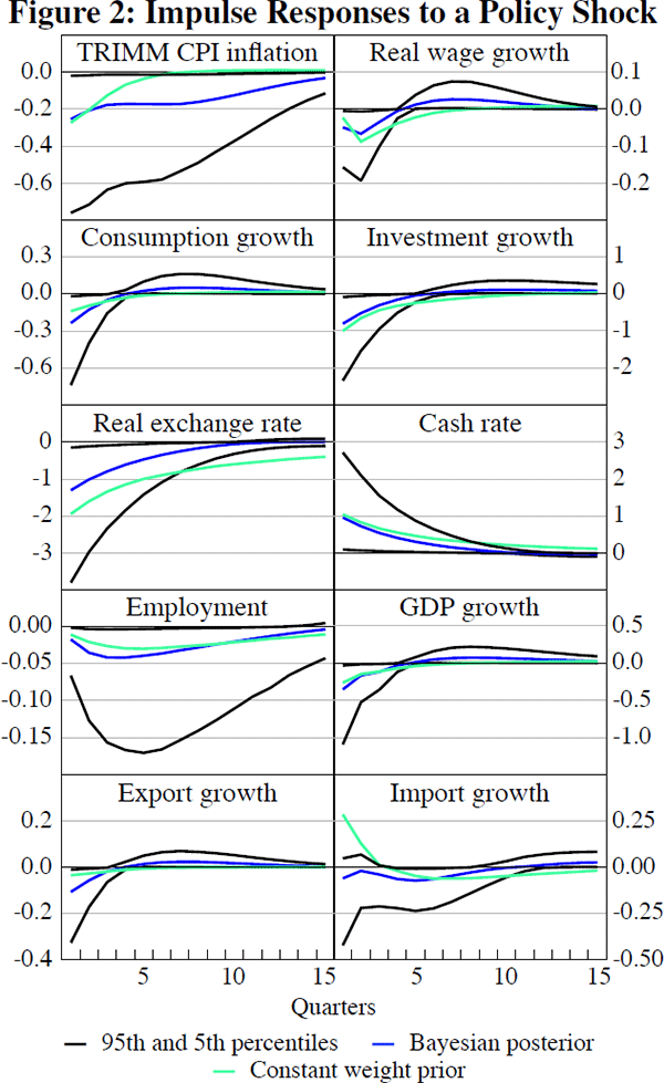
Figure 2 illustrates the dynamic response to a 100 basis points monetary policy shock (median, 5th and 95th percentiles).[8] The main variables respond as we might expect. Consumption and investment decrease, which together with the appreciation of the real exchange rate means that the marginal cost of production and the price of imported goods are falling, which leads to falling inflation. The maximum response of CPI inflation to a unit shock to the interest rate is about 0.3 percentage points.

The magnitude and persistence of the response of CPI inflation to a monetary policy shock is quite sensitive to the prior chosen for the degree of nominal stickiness for domestic consumption goods (as captured by the Calvo parameter). With a very weak prior (or no prior at all) on this parameter, the estimated responses were found to be much more short-lived (the green line in Figure 2 shows the mean response when no prior information was imposed). However, the estimated value of ξd with no prior implied that domestic firms only re-optimise prices every five years, which does not seem realistic. We do think that a prior centred on re-optimisation on average every three quarters is defensible and accordingly, we also think that the implied responses to policy shocks are reasonable.[9]
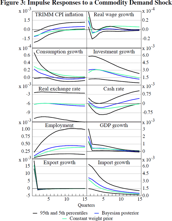
In Figure 3 we plot the impulse responses to a standard deviation shock to commodity demand. An increase in commodity demand generates an output expansion, an increase in employment, and a fall in inflation (at least initially). This last effect is explained by the real exchange rate appreciation, which reduces imported goods inflation, and makes imported capital goods cheaper. The exchange rate effect is strong enough to initially counteract the pressures on marginal cost stemming from the expansion of employment and the increase in real wages and consumption. After about seven quarters though, the response of inflation is positive and quite persistently so.

4.3 Which Shocks are Important?
The model can be used to decompose the causes of the unconditional variances of the
observable variables into their orthogonal components. The result of this
exercise is displayed in Table 3, where we report the variance decompositions
of the 10th, 50th and 90th percentiles of the posterior distribution for selected
observable variables. The shocks are grouped into five categories. The first
contains technology shocks: the stationary (εε,t), unit root (εz,t),
investment-specific (εϒ,t) and asymmetric
technology  shocks. The second category includes ‘supply’
shocks: the labour supply shock
  and shocks to the mark-ups of the domestic
 ,
imported consumption
 ,
imported investment
  and export
  goods. The third category
includes the domestic ‘demand’ shock (the consumption preference
shock,
  ).
The fourth category includes shocks associated with external factors: the
uncovered interest rate parity
  , commodity demand (εcom,t),
commodity price (εpcom,t), foreign output
  ,
foreign interest rate
  and foreign inflation
  shocks. Finally, we
have the monetary policy shocks (εR,t and
  ).
The table excludes shocks that have a small impact on all endogenous variables,
which explains why the fraction of variances explained by the shocks in Table
3 add up to less than 100 per cent.
| Variable | Shock | ||||
|---|---|---|---|---|---|
| Technology | Supply | Demand | External | Monetary policy | |
 |
0.06 | 0.73 | 0.04 | 0.08 | 0.02 |
| (0.01–0.21) | (0.41–1.00) | (0.01–0.27) | (0.03–0.20) | (0.01–0.08) | |
| ΔIn(Wt/Pt) | 0.44 | 0.52 | 0.00 | 0.01 | 0.02 |
| (0.31–0.58) | (0.40–0.67) | (0.00–0.00) | (0.00–0.02) | (0.00–0.06) | |
| ΔIn(Ct) | 0.26 | 0.06 | 0.64 | 0.01 | 0.01 |
| (0.10–0.45) | (0.02–0.15) | (0.40–0.85) | (0.00–0.50) | (0.00–0.03) | |
| ΔIn(It) | 0.20 | 0.30 | 0.01 | 0.42 | 0.01 |
| (0.07–0.44) | (0.11–0.60) | (0.00–0.08) | (0.25–0.60) | (0.00–0.03) | |
 |
0.03 | 0.90 | 0.00 | 0.05 | 0.00 |
| (0.00–0.18) | (0.69–0.98) | (0.00–0.03) | (0.02–0.14) | (0.00–0.00) | |
| Rt | 0.10 | 0.71 | 0.05 | 0.06 | 0.01 |
| (0.02–0.30) | (0.39–0.98) | (0.01–0.28) | (0.03–0.17) | (0.00–0.05) | |
| Et | 0.05 | 0.85 | 0.02 | 0.05 | 0.00 |
| (0.01–0.19) | (0.52–0.97) | (0.00–0.23) | (0.01–0.16) | (0.00–0.00) | |
| ΔInYt | 0.30 | 0.23 | 0.15 | 0.25 | 0.02 |
| (0.15–0.50) | (0.11–0.41) | (0.07–0.30) | (0.14–0.40) | (0.00–0.07) | |
| ΔInXt | 0.27 | 0.22 | 0.00 | 0.48 | 0.00 |
| (0.16–0.41) | (0.12–0.37) | (0.00–0.02) | (0.35–0.63) | (0.00–0.01) | |
| ΔInMt | 0.10 | 0.10 | 0.02 | 0.73 | 0.00 |
| (0.00–0.26) | (0.03–0.21) | (0.01–0.07) | (0.58–0.87) | (0.00–0.01) | |
| Note: Figures in brackets indicate 90 per cent posterior probability intervals. | |||||
It is clear from the table that the world shocks are important drivers of the Australian business cycle: 25 per cent of the variance of non-farm GDP growth; 42 per cent of the variance of investment; and 48 per cent and 73 per cent of export and import growth, respectively, are explained by the external shocks. Of the observed variables, consumption and real wage growth seem to be the domestically most ‘isolated’ variables, with a significant fraction of their variances explained by productivity and supply shocks (within this category the labour supply shock is one of the most important drivers of real wage growth, it explains around 42 per cent of the variance of real wage growth).[10]
The mark-up on the price of imported consumption goods appears to be an important source of CPI inflation volatility. It is estimated to explain about 60 per cent of the variance of CPI inflation.[11]
Turning to the commodity demand shocks, it is worth first noting that these are orthogonal to world output (which is included as a separate observable variable), and will thus not capture increases in demand for Australian exports due to high world output.[12] Exogenous commodity demand shocks appear to have the largest impact on the variance of export growth, explaining about 25 per cent of this variance.
4.4 Outstanding Issues
The model features a single stochastic trend, driven by the permanent technology shock (captured by μz). This implies that real variables (GDP, consumption, investment, imports, exports and the real wage) are non-stationary and grow at the same rate in the long run. The common stochastic trend also means that real variables can be normalised by the technology factor so as to be stationary. We noticed, however, that some of these normalised variables embedded in the state vector ξt exhibit a very persistent, trend-like behaviour within the sample.
In short samples, it may be hard to distinguish a protracted cyclical difference in average growth rates (or structural breaks) from a secular trend in the data. For instance, the growth rates of investment, exports and imports are higher than the average output growth in the sample that we use to estimate the model (and the growth rates of real wages and world output have been lower than non-farm output growth).[13] If this is merely a cyclical difference, one would expect the growth rates of these variables to be lower on average than output growth in the future in order to return the economy to its steady-state growth path. However, if the differences in growth rates reflect a lasting trend, then the model is obviously misspecified. If we believed that this is indeed the case, the difference in growth rates could be removed before estimating the model in order not to force the model to explain a trend in the data as part of the business cycle. It is, however, hard to think of a good reason why investment, for instance, should grow faster than output in the long run.
In the benchmark specification we chose not to adjust the mean growth rates of the real variables, but we also estimated an alternative model with the adjusted data. When we adjusted real variables to grow at the same rate as non-farm output (that is, the data was reconstructed to co-trend), the estimated shocks became less persistent. The drop in persistence was most notable in the asymmetric technology shock, which captures the degree of asymmetry in the growth rates between the domestic economy and the rest of the world, and in the consumption preference shock (which is a demand shock in the model).[14]
Footnotes
Note that there is a difference between price re-optimisation and price re-setting, because there is partial indexation in the model: prices change every quarter for all producers, a fraction ξ because producers re-optimise and a fraction 1 – ξ because of dynamic indexation. [6]
We flag some potential explanations for this in Section 4.4. It is also worth noting that we tried different wage indexation schemes but they did not improve the fit of the real wage series. [7]
A one standard deviation monetary policy shock equals roughly 70 basis points. This is expressed on an annualised basis and recall that data are quarterly. [8]
Del Negro and Schorfheide (2008) report a similar finding. They study the role of nominal rigidities in a New Keynesian DSGE model and find that post-1982 US data cannot discriminate between low- and high-price rigidity specifications. These two different model specifications, however, imply strikingly different dynamic effects of a monetary policy shock. [9]
Nimark (2007) finds that foreign shocks account for 65 per cent, 67 per cent and 58 per cent of the variance of domestic output, inflation, and interest rates, respectively. Medina and Soto (2007) find that foreign shocks explain about 45 per cent of the output variance and about 30 per cent of the inflation variance in the Chilean economy. Interestingly, Justiniano and Preston (2006) fail to identify significant variance shares for foreign shocks in an estimated small open economy for Canada. All of these models, however, abstract from a shock to the level of trend technology and pre-filter data before estimation. [10]
One might have expected a more sizeable role for the exchange rate in driving the volatility of import prices. It may be that the mark-up shock is capturing some volatility that cannot be systematically attributable to the exchange rate. [11]
Caution should be used when interpreting what we have described as the commodity demand shock since in our set-up it may be hard to distinguish this from a supply shock. [12]
See Figure 1. The model consistently overpredicts, for instance, the growth rate of real wages. [13]
We also estimated a closed economy version of the model (which is as presented in Del Negro et al 2007) to see to what extent some of these issues emerge through the open economy part of the model. It turns out that simplifying the model in this way is not very helpful, which is hardly surprising given that we use the same ‘domestic’ real variables (consumption, investment, real wage) as observables as before when estimating the model, and any excessive trend in these variables will just be attributed to any remaining shocks in the theoretical model. [14]