RDP 2008-05: Understanding the Flattening Phillips Curve 3. A Structural Perspective on the Flattening Issue

The problem with the results above is that, because they come from reduced-form regressions, it is hard to tell whether they represent a change in the true responsiveness of inflation to the output gap, as opposed to a change elsewhere in the economy (for example, in the policy rule, if the central bank decided to respond more aggressively to expected inflation). This is just the Lucas critique (Lucas 1976). Consequently, we now turn to more structural estimates of the inflation process. We adopt the common new-Keynesian framework to examine whether a flattening has occurred and, if so, to review its possible causes.

3.1 A Brief Review of New-Keynesian Inflation Theory

The basic idea of the new-Keynesian Phillips curve is that, in an environment in which there are only occasional opportunities to adjust prices, firms will set their prices in anticipation of expected future costs. The key points are that prices are determined by costs (via a desired price/cost mark-up), and that there is a forward-looking element to price setting. For an extensive survey of the literature see Òlafsson (2006).

The canonical expression of this theory is the new-Keynesian Phillips curve,

as derived in Galí and Gertler (1999), where β is the discount factor, mc is the real marginal cost and λ is its coefficient. However, this specification has been found to not capture the observed persistence of inflation. Consequently, it has been generalised by introducing either rule-of-thumb pricing (Galí and Gertler), or indexation (Christiano, Eichenbaum and Evans 2005), both of which have the result of introducing a lag of inflation to the Phillips curve:

This is commonly referred to as the hybrid new-Keynesian Phillips curve, and the γ_f and γ_b coefficients respectively reflect the degree of ‘forward lookingness’ and inertia in inflation.^[5]

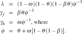
What makes Equation (3) attractive is that it can be derived from explicit microeconomic foundations, such as Calvo pricing (Calvo 1983), as sketched in Galí and Gertler (1999).^[6] Specifically, let θ represent the probability that a firm is unable to adjust its prices in any given period. Furthermore, let ω represent the share of firms who can change their price, but instead of doing so optimally follow a ‘rule of thumb’ and base their price adjustment on lagged inflation, while the remaining 1 − ω set their prices optimally.^[7] In this case, the γ_f, γ_b and λ parameters are functions of the deep parameters ω and θ, and the discount factor β as follows:

It is possible to solve the new-Keynesian Phillips curve forward, for example, using the approach of Binder and Pesaran (1995), which yields:

where and |P| < 1.^[8]

This highlights that, in this framework (abstracting from the lagged inflation term), it is the expected path of current and future real marginal costs that determines current inflation.

Finally, the closed form can be used to see why the reduced-form estimates may not actually correspond to a structural flattening of the Phillips curve. Suppose, just as an illustration, that real marginal costs follows an AR(1) process,

so that

Under this assumption, the closed form of the new-Keynesian Phillips curve can be written very simply as

What is interesting is that, except for the substitution of the real marginal cost mc for the conventional output gap, this is indistinguishable from the reduced-form Phillips curves that are often estimated. As usual, the reduced-form coefficients are complicated functions of the underlying parameters of interest. A flattening of the reduced-form Phillips curve can reflect, in this example, either a change in the slope of the structural Phillips curve (a reduction in λ) or a decrease in the persistence of marginal cost fluctuations. Thus, the reduced-form Phillips curve may flatten for reasons completely unrelated to any structural change in the relationship between prices and marginal costs.

This is not a new idea. Roberts (2006) examines the implications for estimates of the slope of the reduced-form Phillips curve of changes in the monetary policy rule, and finds that more responsive policy could underlie a reduced-form flattening. Similar results were obtained analytically by Carlstrom, Fuerst and Paustian (2007).^[9]

Changes in the link between the output gap and marginal costs are another possible source of change in the relationship between inflation and the output gap. Specifically, if marginal costs become less sensitive to fluctuations in economic activity, then inflation will be less sensitive to the output gap.

Footnotes

Nimark (2008) provides an alternative explanation for the inertia, namely imperfect information about firms' marginal costs. [5]

An alternative approach is to use quadratic adjustment costs; see Rotemberg (1982). [6]

In the steady state there is assumed to be no inflation, although this is relaxed by Ascari (2004), who argues that the assumption is not innocuous. We revisit this in Section 5.4. [7]

Note that this does not guarantee a unique solution. For stability we also need . [8]

Interestingly, Rudebusch (2005) found quantitatively small effects of increasing ‘aggressiveness’ on the reduced-form parameter estimates. [9]