RDP 2008-05: Understanding the Flattening Phillips Curve 2. Reduced-form Flattening

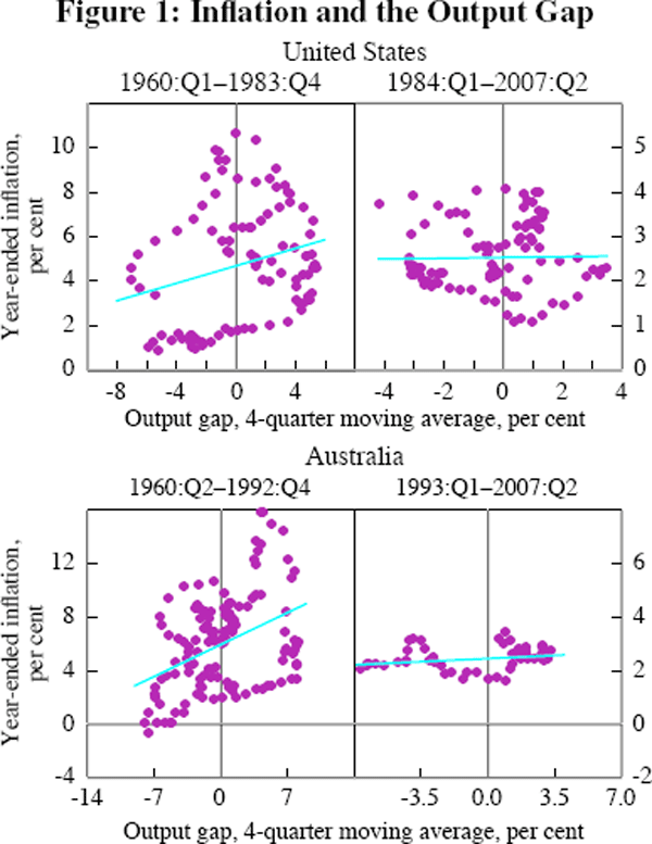
Simple scatterplots of inflation and the output gap are striking (Figure 1). We divide the sample for both countries, with the period after the break displaying a sizeable drop in the volatility of the output gap in each country.^[1] The moderation of the business cycle has been widely studied – see, for example, the papers in Kent and Norman (2005). The accompanying decline in inflation, however, has not been proportional – the reduced-form Phillips curve has flattened.

Reduced-form estimates of the Phillips curve, like those in Roberts (2006), typically have the specification:

where: π_t is quarterly inflation; y_t is an estimate of the output gap; L is the lag operator; and z_t represents some exogenous factors affecting inflation.^[2] The lags of inflation (we use two) are sometimes interpreted as a proxy for inflation expectations, and more generally to capture the observed persistence in inflation.^[3] To examine the flattening of the Phillips curve we want to allow c, the coefficient on the output gap, to vary over time. Two simple ways of doing this are to estimate Equation (1) over a 15-year rolling window (Figure 2), or to specify the process so that the output gap coefficient follows (we assume a random walk) and to use the Kalman filter to estimate it over time (Figure 3). The latter has the advantage that it delivers two-sided estimates, that is, at all points of time they use information from the entire sample.

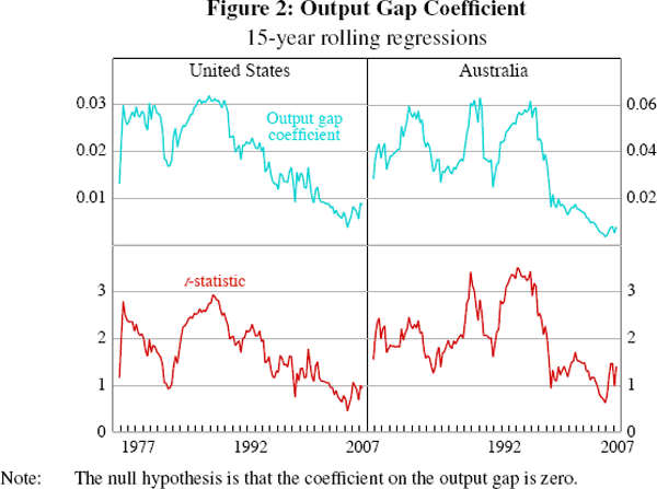
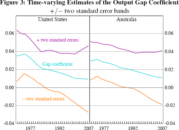
The flattening of the reduced-form Phillips curve is clearly evident for the United States using either methodology. In Figure 2 we date the parameter estimates at the end of each rolling window, and consequently the sharp reduction in the output gap's coefficient evident from around 1989 occurred in the preceding 15 years, and perhaps is better dated in the early 1980s, around the time when the Federal Reserve managed to reduce inflation. Alternatively, the two-sided estimates in Figure 3 suggest that the flattening of the Phillips curve began around 1975 and has been a very gradual process which continued over the 1980s and 1990s.^[4]

The results for Australia are more mixed. The estimates of the coefficient on the output gap fluctuate considerably until the late 1990s, after which there is a clearly discernable downward trend. Once again, this suggests that the flattening began around the time of a change in monetary policy regime, namely the adoption of inflation targeting. The two-sided estimates, however, date the flattening as beginning far earlier, around 1975, akin to the findings for the United States.

Footnotes

The break in 1984:Q1 for the United States follows Roberts (2006). The break in 1993:Q1 for Australia corresponds to the adoption of inflation targeting. The output gap is constructed using a quadratic trend – see Section 4 for further details on the data. [1]

In the rolling regressions we exclude z_t. Including the change in import prices moderates the extent of the flattening evident for the United States, but not for Australia. Adding further lags of inflation or changes in oil prices does not change our results qualitatively. [2]

Often the coefficients on the lags of inflation are restricted to sum to 1 (and the constant restricted to be 0), in an attempt to ensure that the Phillips curve is vertical in the long run (this is the ‘accelerationist’ model of inflation). These restrictions imply that inflation is an integrated process, which is implausible when the central bank's reaction function satisfies the ‘Taylor Principle’, that is, they move the nominal interest rate more than one-for-one in response to expected inflation. They also ignore the cross-equation restrictions that would exist in a fully-specified model – a point first highlighted by Sargent (1971). However, whether the Federal Reserve tightened sufficiently to offset inflation in the 1970s is debatable – see Clarida, Galí and Gertler (2000) and Orphanides (2002). [3]

Naturally, this partially reflects our assumption that the coefficient on the output gap follows a random walk. The start date for the time-varying parameter estimates is 1970:Q1. [4]