RDP 2008-02: Combining Multivariate Density Forecasts Using Predictive Criteria 2. A Suite of Models

The aim of this paper is to construct accurate multivariate density forecasts of GDP growth, inflation and short-term interest rates from a suite of models. We consider three types of models: a BVAR with Minnesota priors, a dynamic factor model or FAVAR and a medium-scale DSGE model. The first two are statistical models with a solid track record in forecasting (see, among others, Litterman 1986, Robertson and Tallman 1999 and Stock and Watson 2002). The structural DSGE model, on the other hand, has a shorter history as a forecasting tool (for examples, see Smets and Wouters 2004; Adolfson, Andersson et al 2005).

All three models restrict the dynamics of the variables of interest in order to avoid in-sample over fitting, which is a well-known cause of poor forecasting performance in unrestricted models (see, for instance, Robertson and Tallman 1999 and references therein). The BVAR shrinks the parameters on integrated variables in an unrestricted VAR towards the univariate random walk model. The FAVAR uses principal components to extract information from a large panel of data in the form of a small number of common factors. The DSGE model uses economic theory to restrict the dynamics and cross-correlations of key macroeconomic time series. Each model is briefly presented below along with an overview of how the individual models are estimated.

2.1 BVAR

The BVAR can be represented as:

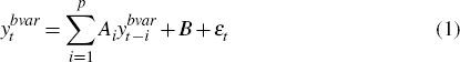
where ε_t ~ N(0,Σ^bvar), B is a vector of constants and is an m × 1 vector that includes quarterly data on the following variables: trade-weighted measures of G7 output growth, G7 inflation and a simple average of US, euro area and Japanese interest rates; the corresponding domestic variables we are interested in forecasting (GDP growth, trimmed mean underlying inflation and the cash rate); and the level of the real exchange rate. Variables in growth rates are approximated by log differences and foreign variables are treated as exogenous to the domestic variables. We consider three specifications of Equation (1) denoted BVAR2, BVAR3 and BVAR4 corresponding to the number of lags p = 2, 3 and 4 respectively.

Minnesota-style priors (Doan, Litterman and Sims 1984; Litterman 1986) are imposed on the dynamic coefficients A_i. The prior mean on the coefficient on the first lag of the dependent variable in each equation is set equal to zero for variables in changes and to 0.9 for the three variables specified in levels (both interest rate variables and the real exchange rate). The prior mean on coefficients for all other lags is set to zero and is ‘tighter’ on longer lags than on short lags. This prior centres the non-stationary domestic and foreign price and output levels on a univariate random walk, and centres domestic and foreign interest rates and the real exchange rate (stationary variables) on AR(1) processes.^[1] A diffuse prior is placed on the deterministic coefficients of the unit root processes and the constants of the stationary processes in B and we impose a diffuse prior on the variance covariance matrix of the errors, p(Σ^bvar) ∝ |Σ^bvar|^−(m+1)/2.

To draw from the posterior distribution of parameters under this Normal-Diffuse prior, the Gibbs Sampler described in Kadiyala and Karlsson (1997) was used, with the number of iterations set at 1,0000 and the first 500 draws used as a burn-in sample to remove any influence of the choice of starting value (the OLS estimate of Σ^bvar was chosen).

2.2 FAVAR

Factor models are based on the idea that a small number of unobserved factors f_t = (f_1t … f_kt)′ can explain much of the variation between observed economic time series. Once estimated, these factors can be included as predictors in an otherwise standard VAR, forming a factor-augmented VAR (see Bernanke, Boivin and Eliasz 2005). The FAVAR therefore takes the same form as Equation (1), where 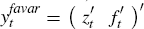and the vector z_t refers to the three domestic variables we are interested in forecasting.

Imposing a diffuse prior on the parameters of the model delivers the standard result that the covariance matrix of the errors Σ^favar is distributed as inverse Wishart (a multivariate generalisation of the inverse gamma distribution), while the regression coefficients follow a normal distribution, conditional on Σ^favar (see, for instance, Kadiyala and Karlsson 1997).

We use principal-components analysis following Stock and Watson (2002) to estimate f_t from a static representation of a dynamic factor model. The static representation is:

where X_t represents a large data panel of predictor variables (demeaned and in stationary form), Λ is a matrix of factor loadings and e_t is an error term (with zero mean) which may be weakly correlated across time and series. The k × 1 vector of static factors f_t can include current and lagged values of the dynamic factors. When lags are included in the dynamic factor representation, the static factors in Equation (2) are estimated by principal components of a matrix that augments the data panel X_t with lags of the data panel. The principal-component estimator of the factors is , where V represents the matrix of eigenvectors corresponding to the k largest eigenvalues of the variance covariance matrix of the data panel (see Stock and Watson 2002 and Boivin and Ng 2005).

The data series included in X_t are the same as in Gillitzer and Kearns (2007) – see Appendix A of that paper for details – except that the three foreign variables used in the BVAR are also included. Up to three static factors (k = 1,2, 3) are included in the model, which are estimated assuming a one-lag dynamic factor model representation. The first three factors explain approximately 25 per cent of the total variation of the data panel. Finally, we allow for either 2 or 3 lags in the FAVAR itself (p = 2, 3), which means that in total, six different specifications of the factor model are considered, each denoted FAVARkp.

One drawback of the principal-components approach is that it gives no measure of the uncertainty surrounding the factor estimates something that could be important for determining the overall uncertainty surrounding the forecasts. Bai and Ng (2006) show that when the number of series included in the data panel n grows faster than the number of observations T (that is T/n → 0), then the impact from using the ‘estimated regressors’ on the variance of the estimated model parameters is negligible. While this condition is not met here, we expect any influence on the variance of the FAVAR's parameters to be factored into the predictive criteria used to combine the different model forecasts.

2.3 DSGE Model

The DSGE model is a medium-scale open economy New Keynesian model that follows the open economy extension of Christiano, Eichenbaum and Evans (2005) by Adolfson et al (2007) closely. It consists of a domestic economy populated with households that consume goods, supply labour and own the firms that produce the goods. Domestic households trade with the rest of the world by exporting and importing consumption and investment goods. Consumption and investment goods are also produced domestically for domestic use. The domestic economy is small compared to the rest of the world in the sense that developments in the domestic economy are assumed to have only a negligible impact on the rest of the world. The model is rich in the number of frictions and shocks, which appears to be important for matching the data.

In order to estimate the model, the structural equations are linearised and the model is then solved for the rational expectations equilibrium. This can be represented as a reduced-form VAR. Since many of the theoretical variables of the model are unobservable, the model is estimated using the Kalman filter. To do this, the solved model is first put in state space form as follows:

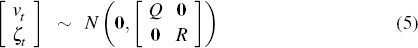
where the theoretical variables are collected in the state vector ξ_t and the observable variables are collected in the vector . The state transition Equation (3) governs the law of motion of the state of the model and the measurement Equation (4) maps the state into the observable variables. The matrices F_ξ, A_X, H′ and Q are functions of the parameters of the model. The observable variables included in are the real wage, real consumption growth, real investment growth, the real exchange rate, the cash rate, employment, real GDP growth, real exports and real imports growth (adjusted), trimmed mean underlying inflation, real foreign (G7) output growth, G7 inflation and the foreign interest rate. Again, variables in growth rates are approximated by log differences.

The covariance matrix R of the vector of measurement errors ζ_t in Equation (4) is chosen so that approximately 5 per cent of the variance of the observable time series are assumed to be due to measurement errors. The model is estimated using Bayesian methods and the posterior distributions of the 52 structural parameters are simulated using 1,000,000 draws from the Random-Walk Metropolis Algorithm, where the first 400,000 are removed as a burn-in sample. Further details of this model are available on request.

Footnote

How strongly the overall and cross-equation elements of this prior are imposed is governed by two hyper parameters which are set at 0.5 and 0.2 respectively. Harmonic lag decay is also imposed. For a useful discussion of the Minnesota prior see Robertson and Tallman (1999). [1]