RDP 2007-07: More Potent Monetary Policy? Insights from a Threshold Model 3. Estimation and Results

The benchmark model is estimated using quarterly Australian data on real GDP growth, CPI inflation, real credit growth and the cash rate over the sample period 1978:Q4 to 2006:Q1.

The length of the moving average (MA) component applied to the credit-growth threshold is allowed to vary from two to four quarters and is determined jointly with its lag length of d (from one to four quarters), and the lag length of the whole system (from one to four quarters). The optimal lag lengths are determined by means of the Schwarz and Akaike information criteria (see Table C1 in Appendix C). The Akaike criterion suggests a two-quarter lag for the whole system (that is, a VAR(2)). The threshold variable is based on a four-quarter moving average of the quarterly growth in real credit (q) with a lag of three quarters. The Schwarz criterion suggested a more parsimonious specification of a one-quarter lag for the system; the choice of q_t−d is, however, in line with the Akaike criterion. I set the number of lags to two according to the Akaike criterion, which also encompasses the lag length of the Schwarz criterion.

The bootstrapped p-value of the sup F test for a threshold model against the baseline alternative of the linear specification is 0.002. Therefore, the hypothesis of linearity in favour of the hypothesis of threshold effects is strongly rejected. Using a linear model in this context may induce misleading conclusions about the general dynamic behaviour of the series, the pattern of the impulse responses and the persistence of the shocks.^[8] The estimated critical value for the threshold variable (based on the MA4, d = 3 quarters specification) is quarterly growth of real credit of 7.7 per cent on an annualised basis; growth rates below this value are assumed to imply less readily available credit. The sample is distributed reasonably evenly between the credit-growth regimes: there are 43 and 68 observations in the low and high regimes, respectively.

Figure 3 plots the deviations of this credit-growth threshold variable from its estimated critical value, and also shows a simple measure of the output gap for comparison (the percentage difference between actual GDP and trend GDP, based on the Hodrick-Prescott filter). Clearly the high-growth regime has been dominant in recent years. Credit growth appears to be broadly pro-cyclical (periods of slower output growth are associated with a negative deviation of the threshold variable from its critical value). So it is not immediately obvious that the threshold variable is doing much more than identifying periods of strong and weak economic activity.

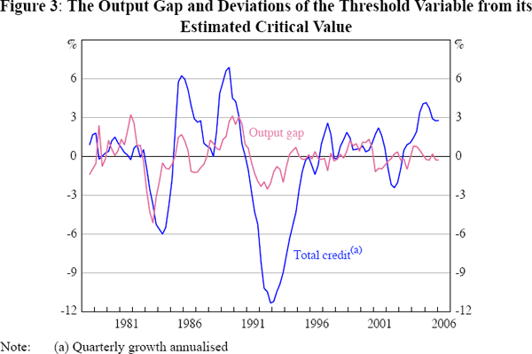
Close inspection of Figure 3 suggests that there have been a number of occasions when the threshold variable based on credit growth has not lined up exactly with the business cycle. In particular, credit growth remained relatively low for a time after recoveries in economic activity following the recessions in the early 1980s and early 1990s. Also, credit growth was especially high during the second half of the 1980s and from 2003 to 2006. 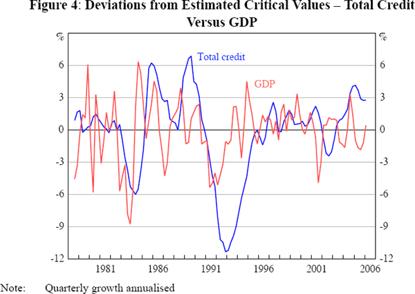It makes sense, therefore, to re-examine the model using GDP growth as the basis for the threshold variable.^[9] Figure 4 shows how the sample is divided into high and low GDP-growth regimes based on a threshold value, , of 3.4 per cent on an annualised basis.^[10] There are some marked differences between the two alternative threshold variables. Perhaps most importantly, compared with the credit threshold variable, the GDP threshold variable switches between regimes with an implausibly high frequency. The GDP threshold variable implies 34 instances of switching compared to only 12 instances for the credit threshold variable.^[11]

3.1 Household and Business Sector Credit

Given the difficulties in determining whether the asymmetries relate to the credit cycle or the business cycle, it may be helpful to repeat the earlier exercise using a separate model for business and household sectors, which have had quite divergent credit cycles. Greater access to credit may help households to smooth consumption, and businesses to take advantage of profitable investment opportunities. So, real household consumption growth is substituted for GDP growth in Equation (2) when analysing household credit, and real business investment is used in the analysis of business credit.^[12]

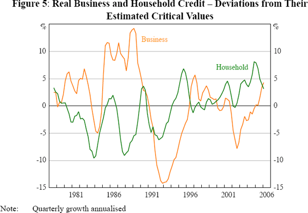
Figure 5 shows the deviations of the household and business real credit-growth threshold variables from their estimated critical values. The critical thresholds for quarterly household and business credit growth are 8.8 per cent and 5.5 per cent, respectively (on an annualised basis). The linearity hypothesis is rejected in both cases.^[13] When credit grows more slowly than these threshold values, credit constraints are likely to be more pervasive than when credit growth is above these values. It can be seen that up to the mid 1990s, except for a few brief instances, household credit growth was below its critical threshold value. However, since then household credit growth has remained, more or less consistently, above the threshold value (there are 55 observations in the low credit-growth regime and 56 in the high credit-growth regime).^[14] Business credit growth shows more volatility, though it crosses its critical threshold less frequently than household credit growth (there are 47 observations below the threshold value and 65 above it). Clearly, the broad changes in credit regimes depicted in Figure 5 are consistent with the discussion above about the timing of apparent credit constraints across the two sectors.

3.2 Impulse Responses across Regimes

Having found evidence of threshold effects, the next step is to calculate the response of GDP to interest rate shocks in each regime, in order to examine the precise nature of the asymmetries. The impulse responses are based on a Cholesky decomposition with the following ordering of variables: GDP growth; inflation; the interest rate; and real credit growth (much of the VAR literature is based on a similar ordering, see, for instance, Leeper, Sims and Zha 1996). Hence, real credit is assumed to react contemporaneously to unanticipated changes in all the other variables in the system, but shocks to credit affect all the other variables with a delay of at least one quarter. The results presented are robust to the alternative ordering of GDP growth, inflation, real credit growth and the interest rate. Although the model is nonlinear, this does not guarantee that the response of the variables to interest rate shocks varies across the two regimes. Figure 6 reports impulse responses for GDP growth following an interest rate shock, conditional on the economy initially being in either the high or the low credit-growth regime.^[15]

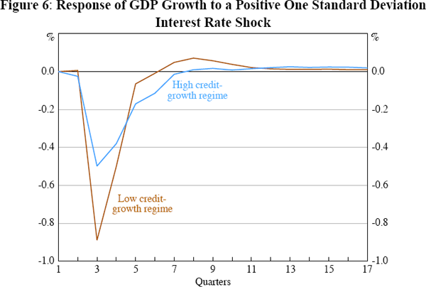
There is clearly evidence of asymmetry across the regimes. The response of GDP growth is considerably larger when the economy is initially in the low credit-growth regime.^[16] The observed pattern of the impulse response for GDP growth is consistent with the predictions of the credit channel model of Bernanke, Gertler and Gilchrist (1999), in which households and business are more affected by a contractionary interest rate shock when they are credit-constrained.^{[17], [18]}

It is worth noting that there is no evidence of asymmetric responses within the regimes: negative and positive interest rate shocks of similar absolute magnitudes have an equal size impact on GDP growth in the opposite direction (results not shown). Moreover, the persistence of positive and negative shocks appears to be roughly the same.

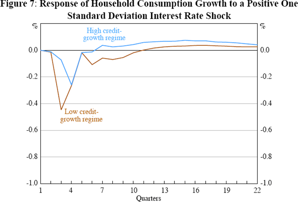
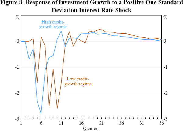
We obtain broadly similar results when the exercise is repeated with alternative model specifications based on either household or business credit. When the growth rate of credit is below the critical threshold value, interest rate movements are more potent. In particular, Figure 7 shows that consumption is more responsive to interest rate shocks when household credit growth is relatively weak, in line with the notion that, at these times, households are less able to smooth consumption in response to temporary shocks.^[19] Also, real business investment shows some signs of being more responsive in the low credit-growth regime (Figure 8). The response of real business investment growth highlights a well-known challenge for modelling short-run movements in investment: investment is especially volatile at a quarterly frequency (Cockerell and Pennings forthcoming). The cumulative effect of a positive interest rate shock on real business investment is, however, negative – and even more so in the low credit-growth regime.

In contrast to the findings based on the credit growth threshold, it is interesting to note that if the (smoothed) growth rate of GDP is used as a threshold variable (see Figure 4), interest rate shocks in the low GDP-growth regime have a somewhat smaller impact than those in the high GDP-growth regime.^[20] The degree of asymmetry between the regimes is, however, negligible and much less pronounced than it is in Figures 6 and 7. This is hardly surprising given the implied frequency of switches between the high and low growth regimes based on GDP growth. This finding can also be taken as evidence that the presence of asymmetry in impulse responses is related to changing credit conditions rather than to the business cycle.

Footnotes

The choice of the model is supported by a likelihood ratio test which finds that the residuals are consistent with white noise. The Q-statistics are not significant for residuals (nor squared residuals), indicating that there is no serial correlation in the residuals. In addition, the residual normality test indicates that the residuals are normal (not reported for brevity). [8]

The information criteria for this model suggest a specification with a lag length of three quarters and a two-quarter moving average of the quarterly GDP growth with a lag of three quarters for the threshold variable. Again, the linearity test strongly rejects the null hypothesis of linearity with a p-value of 0.000. Values for the Akaike and Schwarz information criteria are smaller for the specification based on the credit-growth threshold variable. The R² measures are, however, somewhat higher for the alternative specification using GDP growth as the basis for the threshold, but may reflect overfitting of the model given excessive switching between regimes. Diagnostic tests indicate that the residuals contain no autocorrelation, but there appears to be a problem with excess kurtosis. This leads to rejection of the Jarque-Bera test for normality. [9]

The GDP-growth threshold variable is based on the MA2, d = 3 quarters specification. [10]

Instead of MA smoothing of the growth rate of GDP, one possibility would be to extract the trend using a filter. I repeated the exercise using an output gap measure (obtained with the Hodrick-Prescott filter) in place of GDP growth in Equation (2). As above, two different types of threshold variables were used: the rate of growth in real credit (smoothed with moving average terms) and the output gap (in this case no further smoothing was applied). Using the output gap as the threshold variable, the Akaike criterion suggests a three-quarter lag for the whole system with the threshold variable based on a lag of one quarter. The output gap threshold variable is much less volatile than the GDP growth variable; there are 25 instances of regime-switching instead of 34 with GDP growth. There are 22 switches when credit growth is used as the threshold variable (this system contains a four-quarter lag for the whole system, and the threshold variable is based on the MA2, d = 3 quarters specification). Statistical comparison across two specifications suggests that the credit threshold model is preferred both in terms of the R² measures and the information criteria. [11]

Another possibility is to analyse consumption and residential investment jointly in the household credit model. This specification yields qualitatively similar results with the household credit model based solely on consumption. [12]

Information criteria suggest the consumption-household credit model fits better than the total credit model given in Equation (2), but the fit of the investment-business credit model is worse than that of the total credit model. The diagnostic tests for both alternatives are generally satisfactory, although there is evidence of non-normality of the residuals. [13]

There are 16 observations above the threshold before 1994, and 8 observations below it after 1994. If, instead of breaking the sample into two parts according to this threshold variable, it is arbitrarily split into pre- and post-1994 periods, model diagnostics indicate that this specification is inadequate. So it appears that the threshold model is able to capture some important features of data that could have been overlooked when grouping data arbitrarily and non-statistically. [14]

Note that confidence intervals around the simulated responses are not shown. It is not clear how to compute confidence intervals accurately in nonlinear models that allow for switching regimes (see, for example, Kilian 1998). However, given that the hypothesis of linearity was strongly rejected, this should mean that the two impulse responses shown are likely to be significantly different from each other as well. [15]

Berkelmans (2005) also includes a credit variable in his model. He estimates (linear) impulse responses which show somewhat more persistency than the ones presented here. One obvious reason for this is that he estimates a model with GDP in levels, whereas I consider the growth of GDP. [16]

The robustness of this empirical finding was tested by replacing credit growth with a measure of household gearing (the growth rate in the ratio of debt to disposable income, shown in Figure 1). Following a positive interest rate shock, GDP growth decreases in both regimes, but by much more in the low-gearing regime. [17]

Over the past few years gross national expenditure (GNE) has been growing at a faster rate than GDP. Using GNE instead of GDP in Equation (2) does not alter the result shown in Figure 6: the effect of monetary policy is still stronger during periods when credit growth is low. [18]

The robustness of this finding was tested by estimating a specification based on the sum of consumption and residential investment growth. Following a positive interest rate shock, the sum of consumption and residential investment decreases in both regimes, but by more in the low-gearing regime. [19]

This result is in line with Weise (1999) who finds a larger response in the high output regime for the US. [20]