RDP 2006-05: Optimal Monetary Policy with Real-time Signal Extraction from the Bond Market 3. The Dynamics of the Estimated Model
June 2006
- Download the Paper 223KB
The dynamic implications of allowing the central bank to extract information from the term structure depend on the magnitude of the noise in the bond market. There is little information in the term structure when bond prices are very noisy, and including it in the information set of the central bank then has little effect on the dynamics of inflation and output. It is therefore of interest to quantify the variances in the model. The parameters of the model are estimated by Bayesian methods using quarterly data for the US ranging from 1982:Q1 to 2005:Q4 and for Australia ranging from 1993:Q1 to 2005:Q3. The shorter sample period for Australia is motivated by the fact that Australia experienced a large downward shift in the level of inflation in the early 1990s. Preliminary estimations suggest that including this shift in the sample may bias the results. First, it makes the estimates more sensitive to the detrending method used. Second, including a non-typical period when inflation is brought down by contractionary monetary policy may bias the estimates of the preference parameters of the Reserve Bank of Australia (RBA) to make it appear more averse to inflation volatility than is actually the case.
The interest rates included are the Federal Funds rate and secondary market rates for 6- and
12-month Treasury bills for the US, and the cash rate and the 180-day bank bill rate and the
12-month Treasury bond rate for Australia. For both the US and Australia, non-farm real GDP and
CPI (excluding food and energy) are used as a measure of output and to calculate quarterly
inflation rates. The data were de-trended using the Hodrick-Prescott filter and the first eight
observations were used as a convergence sample for the Kalman filter. The prior modes,
distributions and estimated posteriors are reported in Table 1 together with the prior  and
the likelihood conditional on the data set Z,
  . The
Appendix contains more details on the estimation procedure.
| Parameter | Prior mode | Prior s.e. | Distribution | Posterior US | s.e. | Posterior Australia | s.e. |
|---|---|---|---|---|---|---|---|
| γ | 3 | 0.32 | normal | 3.43 | 0.24 | 3.03 | 0.22 |
| φ | 10 | 1.41 | normal | 8.49 | 0.08 | 9.65 | 0.18 |
| η | 1 | 0.32 | normal | 0.90 | 0.04 | 0.89 | 0.08 |
| θ | 0.75 | 0.11 | beta | 0.93 | 0.06 | 0.80 | 0.04 |
| ω | 0.3 | 0.03 | beta | 0.41 | 0.01 | 0.35 | 0.03 |
| β | 0.99 | 0.02 | beta | 1.00 | 0.012 | 0.99 | 0.10 |
| ρ | 0.8 | 0.28 | beta | 0.82 | 0.007 | 0.92 | 0.11 |
| λy | 0.5 | 0.32 | normal | 0.40 | 0.03 | 0.45 | 0.09 |
| λi | 0.5 | 0.32 | normal | 0.20 | 0.01 | 0.48 | 0.13 |
 |
flat | 3.0×10⁻³ | 0.02 | 1.3×10⁻⁵ | 1.2×10⁻⁴ | ||
 |
flat | 6.9×10⁻⁵ | 1.5×10⁻⁶ | 2.5×10⁻⁵ | 1.1×10⁻⁵ | ||
 |
flat | 2.5×10⁻⁶ | 9.0×10⁻⁷ | 1.3×10⁻⁴ | 4.5×10⁻⁵ | ||
 |
 |
 |
normal | 1.1×10⁻⁴ | 1.2×10⁻⁶ | 7.7×10⁻¹² | 4.2×10⁻⁸ |
 |
 |
 |
normal | 5.0×10⁻¹⁵ | 1.9×10⁻⁶ | 3.9×10⁻⁵ | 2.2×10⁻⁵ |
 |
 |
 |
normal | 4.2×10⁻⁶ | 2.3×10⁻⁶ | 9.5×10⁻⁶ | 3.3×10⁻⁶ |
 |
 |
 |
normal | 3.2×10⁻⁷ | 1.2×10⁻⁷ | 3.7×10⁻⁵ | 1.4×10⁻⁵ |
 |
 |
 |
normal | 1.5×10⁻⁶ | 1.2×10⁻⁶ | 3.9×10⁻⁷ | 1.3×10⁻⁶ |
 |
 |
 |
normal | 4.4×10⁻⁶ | 6.7×10⁻⁷ | 2.2×10⁻⁵ | 5.6×10⁻⁶ |
 |
 |
 |
normal | 5.1×10⁻⁵ | 8.4×10⁻⁶ | 4.8×10⁻⁵ | 1.1×10⁻⁵ |
 |
14.3 | 8.9 | |||||
 |
1915.5 | 848.2 | |||||
 |
1929.8 | 857.2 |
The posterior estimates for the structural parameters governing the behaviour of households and firms are similar across the US and Australia. The higher estimated value of λi indicates that the RBA seems to be smoothing interest rates more than the Federal Reserve.
The measurement error in the short-term interest rate is bounded between zero and 1/100 of the
variance of the short interest rate, reflecting that this is a precise measure of the policy
instrument. The prior distribution of the variance of all other measurement errors are normal,
with means equal to 1/5 of the variance of the corresponding data series. We have two sets of
measurement errors on output and inflation. The measurement errors in the theoretical model
capture the variance of the central bank's misconception of the lagged aggregate variables
and are denoted by  and
and  . The second
set, which are the econometric measurement errors, corresponds to the measurement errors in the
data series that are used to estimate the model. These are denoted by
  and
and
 and
their estimated values are discussed in Section
3.2 in the context of the overall fit of the model. The posterior estimates of the model
measurement errors on lagged output and inflation as well as the non-fundamental shocks in the
term structure, are larger for Australia than for the US, and the consequences of this are
analysed in the next section.
3.1 Impulse Responses and the Role of Term Structure Information
Figures 1 and 2 below illustrate the impulse responses of output, inflation and the short interest rate for the US and Australia to productivity, demand and cost-push shocks.
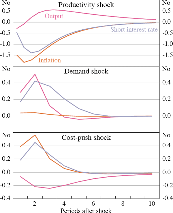
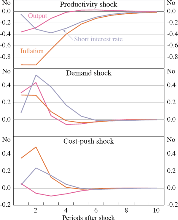
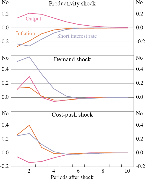
In the US, the short interest rate responds more to the shocks in the impact period than in Australia. Part of this difference can be explained by differences in the informational content of the term structure in the two economies. In Figure 3 the impulse responses to the same shocks as above are plotted for Australia, but with no noise in the term structure. The Australian central bank then has more accurate information and we can see that the responses to shocks are much larger in the impact period. Output now immediately increases in response to a positive productivity shock since short rates fall by more. The Australian central bank can then also counter a cost-push shock by lowering demand already in the impact period.
The analysis above emphasises the beneficial aspects of responding to the term structure, but since the term structure is noisy, this means that sometimes the central bank will inadvertently respond to non-fundamental shocks. The responses of output, inflation and the short interest rate in the US and Australia to a unit non-fundamental shock to the 1-year bond rate are plotted in Figure 4.
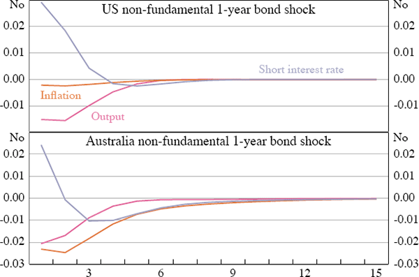
The short interest rate in both the US and Australia increases in response to the non-fundamental shock in the 1-year interest rate, leading to a fall in both output and inflation. The response is quite small for both countries, with a 100 basis point increase in the 1-year yield resulting in an increase of approximately 3 basis points in the short rate. The increase in the short rate leads to lower output and inflation.
3.2 The Fit of the Model
In order to assess the fit of the model, we can look at the estimated variances of the errors in the empirical measurement equation. Table 2 reports the ratio of the variance of the measurement errors in the observation over the variance of the corresponding variable for both the US and Australia. A large value indicates that the model is not very good at explaining the movements of the corresponding observed variable, since that means that a large portion of the variance of the variable does not conform to the model's dynamic and cross-equational implications. In general, the fit of the model is worse for Australia than for the US. There may be several explanations for this finding. First, Australia is a small, open economy while the US is a large and relatively more closed economy. This means that the baseline closed-economy New-Keynesian model employed here may be too simple to capture the dynamics of the Australian economy. The Australian economy is likely to be more affected by terms of trade shocks and shocks that affect capital flows and the exchange rate. As far as the responses of the endogenous variables to these types of disturbances are not nested in the demand, cost-push and productivity shocks of the model, this will reduce the fit. Another possible explanation, at least for the worse fit of long interest rates, is that the Australian bond market is not as deep as the US bond market. With fewer traders active, the market may be less efficient at aggregating dispersed information.
| US | Australia | |
|---|---|---|
 |
0.0099 | 0.24 |
 |
0.010 | 0.22 |
 |
0.010 | 0.0008 |
 |
0.011 | 0.31 |
 |
0.354 | 0.60 |
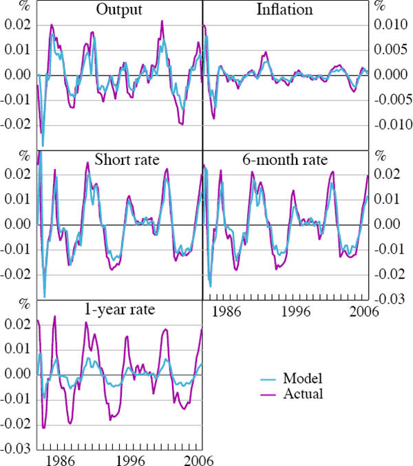
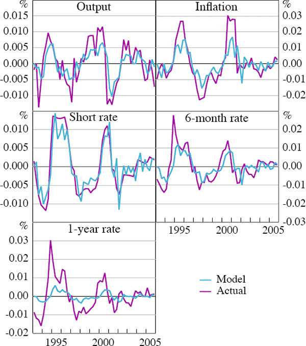
Figures 5 and 6 plot the actual data series and the model's fitted series of the observable endogenous variables. The model does a good job at tracking output, inflation, the short interest rate and the 6-month yield in the US, but has problems matching the volatility of the 1-year yield. The dual of the model's inability to match the long rate is that the long rate does not provide a lot of information about the underlying state of the model. The fit of the model is overall worse for Australia.
3.3 Variance Decomposition
The estimated model can be used to decompose historical variances of the endogenous variables into their exogenous sources. Table 3 reports the results of this exercise. In the US, inflation variance is driven almost entirely by cost-push shocks. The two main sources of fluctuations in output are productivity shocks and non-fundamental shocks to the 6-month bond rate, with respective shares of 77 per cent and 19 per cent. The proportion of variation attributed to non-fundamental sources may seem large. The present model attributes monetary policy shocks, that is, non-systematic movements in the interest rates to misconceptions about the state of the economy on behalf of the central bank, and thus gives a clear interpretation of the policy shock. From this perspective, 19 per cent is comparable to that found by other studies, where the central bank is assumed to be perfectly informed (for example Smets and Wouters 2004). That the ‘policy shocks’ appear to come from the bond market suggests that the misconceptions about the state of the economy may have been shared by the bond market participants. More than half of the variance of the US policy instrument is in response to productivity and demand shocks. That demand shocks explain only a small fraction of inflation and output variation suggests that these responses have been quite successful. About 20 per cent of the interest rate variance is explained by the non-fundamental shock to the 6-month interest rate. The instrument is the channel through which these shocks feed into the economy, and it may appear as if responding to these shocks is not optimal. However, since the central bank is assumed to respond with statistically optimal weights to movements in the term structure, the benefits of having more accurate estimates of the state, on average, outweighs the cost of occasionally responding to ‘false alarms’.
 |
 |
 |
 |
 |
 |
 |
 |
|
|---|---|---|---|---|---|---|---|---|
| US | ||||||||
| yt | 0.77 | 0.04 | 0 | 0 | 0 | 0 | 0.19 | 0 |
| πt | 0.10 | 0.03 | 0.84 | 0 | 0.02 | 0 | 0.01 | 0 |
| it | 0.35 | 0.42 | 0 | 0 | 0 | 0 | 0.20 | 0 |
| Australia | ||||||||
| yt | 0.01 | 0.75 | 0.10 | 0.01 | 0.03 | 0 | 0.10 | 0 |
| πt | 0.02 | 0.01 | 0.94 | 0 | 0.02 | 0 | 0.01 | 0 |
| it | 0.02 | 0.32 | 0.35 | 0.03 | 0.10 | 0 | 0.17 | 0.01 |
The variance decomposition for Australia has a quite different pattern. Productivity shocks seem to play a very limited role for output, inflation and interest rate variances. A large portion of output-gap variance (75 per cent) is driven by demand shocks, and they also explain about a third of the variance of the short interest rate. Inflation is almost entirely explained by cost-push shocks. Central bank misconceptions of the inflation rate explains 10 per cent of the short interest-rate variance while noise in the 6-month rate explains about 17 per cent. The responses of monetary policy to these non-fundamental shocks in turn explains 10 per cent of the variance of output.
3.4 Robustness
In the baseline estimation above it was assumed that the central banks had an explicit interest rate smoothing objective. An alternative explanation of inertial interest rate changes is that central banks move slowly because they want to accumulate more information before they move. The model was re-estimated after imposing no interest rate smoothing, that is, by setting λi = 0. This leads to large reductions in the posterior probabilities for both the US and Australia, and the corresponding posterior odds ratios do not support the hypothesis that λi = 0.[5]
In the estimation, it was also imposed that the central banks of both the US and Australia used the information in the term structure to set policy. If this assumption is incorrect, it would bias the estimates of the noise in the term structure upwards. The log likelihood for both the US and Australia decreases slightly when we re-estimate the model without assuming that the central banks use the information in the term structure. The change for the US is slightly larger, probably because the assumption that the central bank observes the term structure should make less of a difference for Australia where the term structure is relatively more noisy.
Footnote
More details on posterior mode estimates and likelihoods for the alternative specifications are available from the author upon request. [5]