RDP 2006-05: Optimal Monetary Policy with Real-time Signal Extraction from the Bond Market Appendix A: The Model

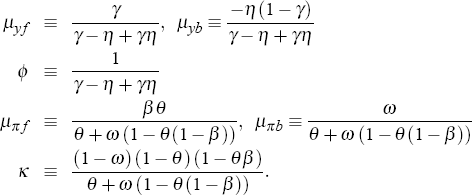
The parameters of the linearised model

are given by

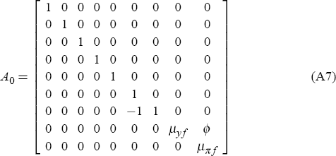
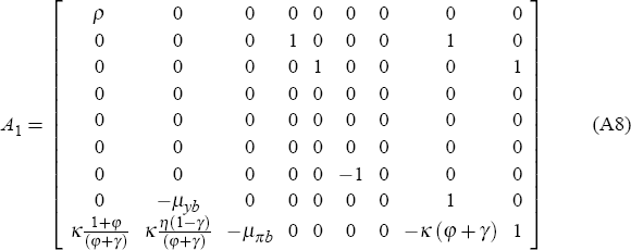
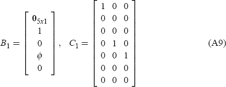
The model can be put in compact form

where the coefficient matrices A, B and C are given by

The likelihood function

To compute the likelihood of the model, we follow the method of Hansen and Sargent (2004). Form a state space system of the AR(1) process of the state

where is the vector of variables that are observable (to us as econometricians) and is the covariance matrix of the econometric measurement errors on output and inflation. Construct the innovation series from the innovation representation

by rearranging to

where K is the Kalman gain matrix

The log likelihood of observing the data Z for a given set of parameters Θ can then be computed as

where

The posterior mode is then given by

where denotes the log of the prior likelihood of the parameters Θ. The posterior mode was found using Bill Goffe's simulated annealing minimiser (available at <http://cook.rfe.org/>). The posterior standard errors was calculated using Gary Koop's Random Walk Metropolis-Hastings distribution simulator (available at <http://www.wiley.co.uk/koopbayesian>).