RDP 2003-11: How Should Monetary Policy Respond to Asset-Price Bubbles? 2. Model

Our model is an extension of the Ball (1999) model for a closed economy. In the Ball model, the economy is described by two equations:

where y is the output gap, r is the difference between the real interest rate and its neutral level, π is the difference between consumer-price inflation and its targeted rate, and α, β, and λ are positive constants (with λ < 1 so that output gaps gradually return to zero).

The Ball model has the advantage of simplicity and intuitive appeal. It makes the simplifying assumption that policy-makers control the real interest rate, rather than the nominal one. It assumes, realistically, that monetary policy affects real output, and hence the output gap, with a lag, and that the output gap affects inflation with a further lag. The values for the parameters α, β, and λ that Ball chooses for the model, and that we will also use here, imply that each period in the model is a year in length.^[2]

We augment the model with an asset-price bubble. We assume that in year 0, the economy is in equilibrium, with both output and inflation at their target values, y₀ = π₀ = 0, and that the bubble has zero size, α₀ = 0. In subsequent years, we assume that the bubble evolves as follows:

Thus, in each year, the bubble either grows by an amount, γ_t > 0, or bursts and collapses back to zero. For ease of exposition, in the rest of this section we will assume that γ_t is constant, γ_t = γ, but we will allow for a range of alternative possibilities in the results we report in Section 3. We also assume that once the bubble has burst, it does not re-form. To allow for the effect of the bubble on the economy, we modify Ball's two-equation model to read:

In each year that the bubble is growing it has an expansionary effect on the economy, increasing the level of output, and the output gap, by γ. The bubble is, however, assumed to have no direct effect on consumer price inflation, although there will be consequences for inflation to the extent that the bubble leads the economy to operate with excess demand as it expands, and with excess supply when it bursts.

When the bubble bursts, the effect on the economy is of course contractionary – if the bubble bursts in year t, the direct effect on output, and the output gap, in that year will be Δα_t = −(t − 1)γ. Thus, the longer the bubble survives, the greater will be the contractionary effect on the economy when it bursts.

We will assume that the evolution of the economy can be described by this simple three-equation system (Equations (3), (4) and (5)). But we distinguish between two policy-makers: a sceptic who doesn't try to second-guess asset-price developments, and an activist who believes that she understands enough about asset-price bubbles to set policy actively in response to them.^[3]

We assume that the policy-makers observe in each year whether the bubble has grown further, or collapsed, before setting the interest rate for that year. Given the nature of the lags in the model, this year's interest rate will have no impact on real activity until next year, and on inflation until the year after that.

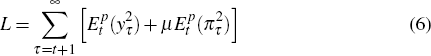
We also assume that the two policy-makers have the same preferences, and that they care about the volatility of both inflation and output. Thus we assume that in each year t, policy-maker p (activist or sceptic) sets the real interest rate, r_t, to minimise the weighted sum of the expected future squared deviations of inflation and output from their target levels, or in symbols, sets r_t to minimise

where µ is the relative weight on the deviations of inflation and is the year t expectation of policy-maker p. In the results we show in the paper, we set µ = 1, so that policy-makers are assumed to care equally about deviations of inflation from target and output from potential.

In setting policy each year, the sceptical policy-maker ignores the future stochastic behaviour of the bubble. Since certainty equivalence holds in the model in this setting, Ball (1999) shows that, for the assumed parameter values, optimal policy takes the form

which is a more aggressive Taylor rule than the ‘standard’ Taylor rule introduced by Taylor (1993), r_t = 0.5y_t + 0.5π_t.

As the bubble grows, the sceptical policy-maker raises the real interest rate to offset the bubble's expansionary effects on the economy. But she does so in an entirely reactive manner, ignoring any details about the bubble's future evolution. Once the bubble bursts, output falls precipitously and the sceptical policy-maker eases aggressively, again in line with the dictates of the optimal policy rule, Equation (7).^[4]

We assume that the activist policy-maker learns about the bubble in year 0, and hence takes the full stochastic nature of the bubble into account when setting the policy rate, r_t, from year 0 onwards. Once the bubble bursts, however, there is no further uncertainty in the model, and the activist policy-maker simply follows the modified Taylor rule, Equation (7), just like the sceptical policy-maker.

Footnotes

Ball's parameter values are α = 0.4, β = 1 and λ = 0.8. Ball also adds white-noise shocks to each of his equations, which we have suppressed for simplicity. [2]

To draw the distinction more precisely, both policy-makers understand how the output gap and inflation evolve over time, as summarised by Equations (4) and (5). The activist also understands, and responds optimally to, the stochastic behaviour of the bubble, as summarised by Equation (3). The sceptic, by contrast, responds to asset-bubble shocks, Δα_t, when they arrive, but assumes that the expected value of future shocks is zero. [3]

We implicitly assume that the zero lower bound on nominal interest rates is not breached when policy is eased after the bubble bursts, so that the real interest rate can be set as low as required by Equation (7). [4]