RDP 2003-11: How Should Monetary Policy Respond to Asset-Price Bubbles? Appendix D: Some Technical Results Required in Appendix C

In this Appendix we set out a number of technical results which we called upon but did not justify in Appendix C, so as not to interrupt the flow of the discussion.

D.1 How the Infinite Loss Horizon is Handled in Appendix C

Recall that the loss function used in the main body of the paper is

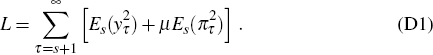
In each period s, this combines contributions from each period of the infinite horizon {s + 1,s + 2,…}. In Appendix C, however, this loss is computed using finite dimensional matrix algebra involving the matrices .

To understand how this is done, the key observation is that, once a bubble has burst, no further shocks are expected to hit the economy. Then, if the bubble bursts in period s + k, it is well known (see (Ball 1999)) that, to minimise L, the optimal setting for policy, in period s + k and all subsequent periods {s + k + 1, s + k + 2,…}, is given recursively by

where the scalar q is defined by q = (− µα + (µ² α² + 4µ)^1/2)/2. Note that Equation (7) is just a special case of this general formula, for the case λ = 0.8, α = 0.4, β = 1 and µ = 1.

Using this, it turns out that, for the case of a bubble which bursts in period s + k, it is possible to express the total contribution to the loss function L, from all periods t > s + k, purely in terms of the values of y and π in period s + k. The precise result, the proof of which is available from the authors upon request, is as follows.

Result 1. Consider an activist policy-maker in period s, facing an asset-price bubble which is expected to burst in period s + k, after which no further exogenous shocks are expected to strike the economy. Then the quantity

satisfies that

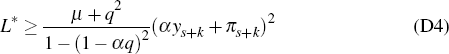
with equality if and only if policy, in all periods t ≥ s + k, is set according to the recursive rule given by Equation (D2).

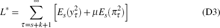
It is now easy to see how the use of the infinite horizon loss function, Equation (D1), is accommodated within the theoretical framework of finite dimensional matrix algebra used in Appendix C. For consider an activist policy-maker in period s facing an asset-price bubble which has not yet burst. As in Appendix C, let denote the contingent loss such a policy-maker would expect were the bubble expected to burst in period s + k. Then, in view of Result 1, we clearly have that in this setting, and with policy for t ≥ s + k set according to Equation (D2),

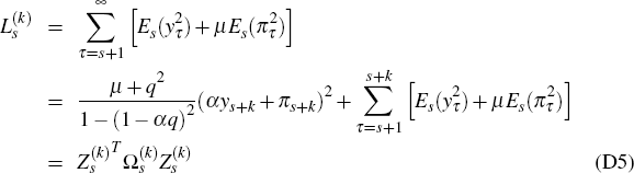
where and are as defined in Section C.3 of Appendix C; and this completes the justification of Equations (C13) and (C14).

D.2 A Matrix Algebra Result

In Section C.5 of Appendix C we also invoked the following linear algebra result.

Result 2. For any period s let the matrices P and Ω_s, and the vector χ_s, be as defined in Appendix C. Next, let V denote the N_s × 1 vector

Then there is a simple formula for V(1), the first component of this vector V, in terms of: the bubble's expected growth next period if it survives, γ_s+1; its current

size 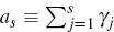; and the probability, , that it will burst in period s+1, given that it has not done so by period s. This formula is

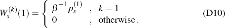
Proof: The proof of this result is quite lengthy and technical. It is available from the authors upon request. The basic idea, however, is first to establish that we may re-write the vector V in the form

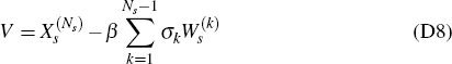
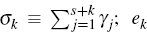
where is as given by Equation (C11), and where, for each k = 1,…,N_s − 1: σ_k denotes the quantity denotes the N_s × 1 vector (0,…, 0, 1, 0,…, 0)^T, the ‘l’ appearing in the k^th entry; and denotes the vector

It then follows directly from Equation (D8) that, to obtain Equation (D7), it will suffice to prove the general formula that, for any k = 1,…, N_s − 1:

Finally, this latter result may be established by: first re-casting the vector quantities as arising from a loss minimisation problem, analogous to the way that the vector V did in Appendix C; and then making a judicious ‘change of variables’ with respect to which to carry out the loss minimisation – a change of variables prompted by the structure of the Ball model.^[27] QED

Footnote

Specifically, recall that in the Ball model changes in interest rates flow through to inflation (via output) with a lag of two periods. Hence, the following two options are readily seen to be equivalent: on the one hand, determining an optimum profile for interest rates, r_t, in periods t = s, s + 1,…, 13, so as to minimise a given loss function; and on the other, seeking instead an optimum profile for inflation, π_t, in periods t = s + 2, s + 3,…, 15, so as to minimise this loss, and then recursively back-solving for the corresponding implied profile for . It is this latter approach which we employ. [27]