RDP 2003-04: Identifying the Efficacy of Central Bank Interventions: Evidence from Australia 5. Results
April 2003
- Download the Paper 129KB
Before we present our results, it is illustrating to demonstrate the problems in estimation that arise from using more traditional methods. As noted earlier, researchers frequently exclude the contemporaneous impact of intervention in an attempt to overcome the endogeneity. To account for the properties of exchange rate data, a GARCH error structure is typically used. Table 3 presents the results from an EGARCH(1,1) model of log changes in the AUD/USD exchange rate over the full sample, and in each of the high- and low-bound regimes. To highlight the impact of the simultaneity bias, we also present regressions that include the contemporaneous intervention. The coefficients on lagged intervention are uniformly small (around 0.005), and frequently the wrong sign, suggesting that RBA purchases of Australian dollars depreciated the exchange rate.
| Full sample | Low-bound regime | High-bound regime | ||||||
|---|---|---|---|---|---|---|---|---|
| (07/1986–11/1993) | (07/1986–09/1991) | (10/1991–11/1993) | ||||||
| Constant | 0.000 (0.000) |
0.000 (0.000) |
0.000 (0.000) |
0.000 (0.000) |
0.000 (0.000) |
0.000 (0.000) |
||
| INTt | −0.016 (0.001) |
−0.020 (0.001) |
−0.012 (0.001) |
|||||
| INTt−1 | 0.004 (0.001) |
−0.003 (0.001) |
0.009 (0.002) |
0.002 (0.002) |
0.000 (0.001) |
−0.002 (0.001) |
||
| INTt−2 | 0.005 (0.001) |
0.002 (0.002) |
0.004 (0.002) |
0.002 (0.002) |
0.005 (0.002) |
0.004 (0.002) |
||
| Constant | −0.904 (0.115) |
−0.807 (0.105) |
−1.331 (0.164) |
−1.316 (0.154) |
−20.122 (0.405) |
−19.373 (0.667) |
||
| |εt−1/σt−1| | 0.286 (0.025) |
0.250 (0.024) |
0.349 (0.035) |
0.333 (0.033) |
0.166 (0.049) |
0.213 (0.071) |
||
| εt−1/σt−1 | −0.053 (0.014) |
−0.049 (0.012) |
−0.083 (0.019) |
−0.085 (0.018) |
−0.053 (0.021) |
−0.061 (0.031) |
||
 |
0.934 (0.010) |
0.940 (0.009) |
0.896 (0.015) |
0.895 (0.014) |
−0.865 (0.038) |
−0.803 (0.064) |
||

|
||||||||
The coefficient on contemporaneous intervention is always significant and incorrectly signed. The estimates are around −0.016 which in absolute value is much larger than the coefficients on lagged intervention. The wrong sign is a direct consequence of the endogeneity. The OLS estimate is a combination of α and β, and likely γ, and can be negative even for positive α if the RBA leans against the wind (β < 0), or common shocks affect the two equations with different signs (γ < 0).[16]
5.1 Contemporaneous Effects of Central Bank Intervention
We now move on to the results from our basic model (Equation (10)) that excludes lags. This implies that the central bank target is the previous day's exchange rate, although the rich error structure will capture deviations from this. Later, we extend the model to include lags which imply a target of a longer moving average.
In Table 4 we report the coefficients of interest: α, β, γ, the two thresholds, the constants and the variances. The first column is the point estimate using the simulated GMM methodology and the moments from the data. The second column is the mean of the bootstrapped distribution of the parameter. As mentioned before, we generate 100 sets of moments bootstrapping the residuals of the original data in each of the regimes. The standard deviation is of the boostrapped distribution of parameter estimates. The fourth column is the quasi t-statistic calculated as the mean divided by the standard deviation. It is important to highlight that the distributions are not normal, so this statistic should be considered informative but not conclusive in terms of the significance of the coefficients. The fifth and sixth column are the maximum and minimum values of the boostrapped estimates. The last column is the percentage of the observations that are below zero. This is the statistic that we use to determine the significance of the coefficients. We prefer to look at the mass above and below zero (these are p-values) rather than the quasi t-statistic, given that most of the estimates are not normally distributed.
| Point estimate |
Mean |
Standard deviation |
Mean/standard deviation |
Maximum |
Minimum |
Percentage of observations below zero | |
|---|---|---|---|---|---|---|---|
| Exchange rate equation | |||||||
| α | 0.1350 | 0.1364 | 0.0372 | 3.66 | 0.2313 | 0.0332 | 0.0 |
| γ | −0.3042 | −0.3054 | 0.0561 | −5.44 | −0.1457 | −0.4481 | 100.0 |
| ce | 0.0043 | 0.0078 | 0.0188 | 0.41 | 0.0904 | −0.0859 | 9.9 |
| Reaction function | |||||||
| β | −0.0279 | −0.0894 | 0.0952 | −0.94 | −0.0047 | −0.5774 | 100.0 |
| cINT | −0.0909 | −0.1104 | 0.0552 | −2.00 | 0.0232 | −0.3580 | 99.0 |
| Other parameters | |||||||
 |
0.3160 | 0.3511 | 0.0869 | 4.04 | 0.9906 | 0.2112 | 0.0 |
 |
1.8529 | 1.9767 | 1.9874 | 0.99 | 21.6319 | 1.2606 | 0.0 |
 |
0.0345 | 0.0159 | 0.0142 | 1.12 | 0.0383 | 0.0000 | 0.0 |
 |
0.4395 | 0.5025 | 0.1837 | 2.73 | 1.3248 | 0.2381 | 0.0 |
 |
0.4094 | 0.4562 | 0.1825 | 2.50 | 1.2857 | 0.0652 | 0.0 |
Our main focus is on the estimate of α. The point estimate is 0.135 and the mean of the distribution is 0.136. The standard deviation is 0.037. Indeed, as can be seen from all 100 realisations, the minimum is 0.033, which implies that there is no mass below zero. Both the quasi t-statistic and the lack of realisations below zero indicate that the estimate is highly significant. The distribution of α is shown in Figure 2.
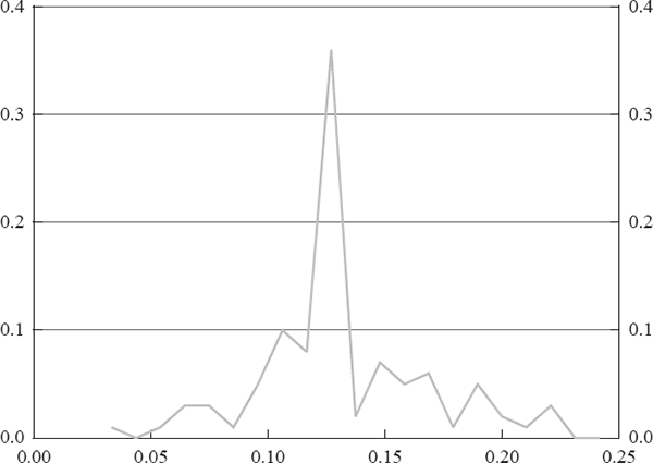
This estimate of α indicates that intervention has a large effect on the exchange rate. The coefficient on contemporaneous intervention, α (0.136), implies that A$100 million of purchases of Australian dollars is associated (on average) with a 1.36 per cent appreciation of the Australian dollar. If we take the average exchange rate over our sample period to be 0.75, then US$100 million of purchases of Australian dollars would have appreciated the Australian dollar by approximately 1.81 per cent. This response is larger than most results in the literature but closely related to calibrations obtained by Dominguez and Frankel (1993c). Dominguez and Frankel calculated that US$100 million of purchases of US dollars would appreciate the US dollar by just under 1.6 per cent.
Our estimate differs from that in Dominguez and Frankel (1993c) in that it is calculated directly from exchange rate and intervention data. In constructing their estimate Dominguez and Frankel need to make several assumptions, such as mean-variance preferences of investors, and use expectations survey data and assets supplies data that are likely to contain measurement errors. The dependence on survey data also requires that they consider exchange rate returns over a longer horizon and so can't estimate the short-run impact of intervention. A significant improvement of our estimation methodology is that we are able to include both contemporaneous intervention and exchange rate returns to address the simultaneity. Nevertheless, our estimate is close to the one found by Dominguez and Frankel (1993c), and we cannot reject the hypothesis that they are the same.
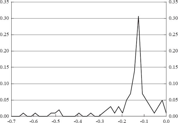
The point estimate of β is −0.028, with mean of −0.089 and a relatively large standard deviation of 0.095. As can be seen in Table 4, the quasi t-statistics suggest that the estimate is not statistically significant from zero. However, demonstrating the importance of the non-normality of the distribution, all realisations are below zero indicating the estimate is highly significant. Figure 3 depicts the distribution of β. As can be seen, the distribution is not normal and there are some realisations that are relatively close to zero, but the distribution has a long left tail.
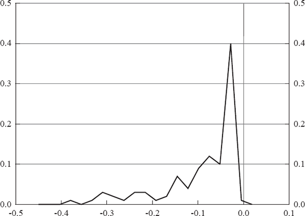
The negative coefficient conforms with our priors, and RBA statements, that interventions are dictated by leaning against the wind. The point estimate implies that in response to a one per cent unexpected depreciation of the exchange rate the central bank will be inclined to lean against the wind, with shadow intervention of a A$0.28 million purchase of Australian dollars to slow the depreciation.
The parameter γ is precisely estimated; it is negative and significant. The point estimate is −0.304, almost identical to the mean of the bootstrapped distribution, −0.305, while the standard deviation is 0.056. In this case, 100 per cent of the bootstrapped estimates are negative, implying that the coefficient is significantly different from zero at high levels of significance. The negative sign of γ demonstrates that shocks common to the exchange rate process and the central bank's reaction function simultaneously weaken (strengthen) the currency and increase (decrease) the central bank's desire to support the currency. Again, this supports our priors of central bank policy. These shocks can be interpreted to be shocks to the exchange rate during periods of high conditional volatility which the central bank shows greater inclination to resist. The negative estimate of γ provides an additional reason why failing to account for the simultaneity of exchange rate and intervention determination is likely to bias downward the impact of intervention on the exchange rate.
Finally, the estimates of the thresholds are highly significant and reasonable given what we have observed. Accounting for the scaling of the data, the thresholds imply that in the early period the central bank participates in the foreign exchange rate market when the shadow intervention is larger than A$3.2 million, while in the later regime it intervenes if the required intervention is larger than A$18.5 million.
5.2 Dynamic Impact of Central Bank Intervention
We now extend the model to allow for two lags in the structural equations. Doing so provides a richer representation of the policy function and allows us to examine the temporal impact of interventions on the exchange rate.
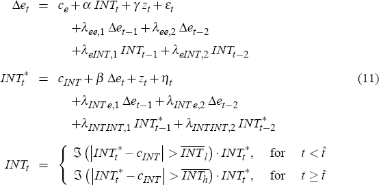
The expanded model is:
where the additional coefficients are the λ's. There are 14 coefficients to be estimated. As noted before, there are 24 moments including the across-time statistics. The results from the estimation are shown in Table 5.
| Point estimate |
Mean |
Standard deviation |
Mean/standard deviation | Maximum |
Minimum |
Percentage of observations below zero | |
|---|---|---|---|---|---|---|---|
| Exchange rate equation | |||||||
| α | 0.0446 | 0.0533 | 0.0375 | 1.42 | 0.1579 | 0.0011 | 0.0 |
| γ | −0.0612 | −0.1400 | 0.0844 | −1.66 | 0.0021 | −0.4130 | 99.0 |
| λee1 | −0.0638 | −0.0603 | 0.0348 | −1.73 | −0.0263 | −0.3196 | 100.0 |
| λee2 | −0.0379 | −0.0385 | 0.0326 | −1.18 | 0.0085 | −0.2962 | 99.0 |
| λelNT1 | 0.0369 | −0.0007 | 0.0351 | −0.02 | 0.0866 | −0.0856 | 65.0 |
| λelNT2 | 0.0246 | 0.0021 | 0.0321 | 0.07 | 0.1060 | −0.0844 | 57.0 |
| Ce | 0.0004 | 0.0100 | 0.0475 | 0.21 | 0.2608 | −0.1263 | 32.0 |
| Reaction function | |||||||
| β | −0.0657 | −0.1538 | 0.1142 | −1.35 | 0.0000 | −0.6292 | 100.0 |
| λINTe1 | 0.0140 | −0.0184 | 0.0186 | −0.99 | 0.0604 | −0.0742 | 87.0 |
| λINTe2 | −0.0030 | −0.0189 | 0.0149 | −1.27 | 0.0760 | −0.0558 | 94.0 |
| λINTINT1 | −0.2299 | −0.0173 | 0.1499 | −0.12 | 0.2819 | −0.6120 | 43.0 |
| λINTINT2 | −0.0923 | −0.0155 | 0.1064 | −0.15 | 0.1913 | −0.3556 | 48.0 |
| CINT | −0.0854 | −0.1933 | 0.1150 | −1.68 | 0.0636 | −0.6258 | 98.0 |
| Other parameters | |||||||
 |
0.3253 | 0.4194 | 0.1007 | 4.16 | 1.0285 | 0.2500 | 0.0 |
 |
2.6664 | 1.6935 | 0.4353 | 3.89 | 2.7410 | 0.7022 | 0.0 |
 |
0.0128 | 0.0062 | 0.0046 | 1.36 | 0.0200 | 0.0000 | 0.0 |
 |
0.3423 | 0.6430 | 0.1495 | 4.30 | 0.9579 | 0.2443 | 0.0 |
 |
0.3044 | 0.4392 | 0.1283 | 3.42 | 0.7659 | 0.0895 | 0.0 |
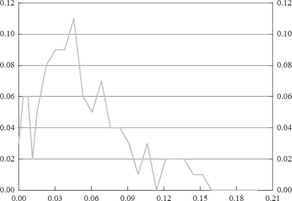
The estimates of α and β have the same signs as those in the base model. The coefficient α is smaller but the coefficients on lagged interventions, λeINT,1 and λeINT,2 are also positive, indicating that intervention continues to affect the exchange rate on the days subsequent to the intervention. Notably, these subsequent effects are smaller. The largest impact from an intervention occurs on the day it is conducted. The coefficient β is again negative, though larger in magnitude. The importance of accounting for the endogenous relationship is highlighted by the much smaller role that exchange rate changes from previous days have in determining intervention, as seen by the small coefficients on lagged exchange rate returns. The coefficients on lagged intervention are negative due to the tendency of subsequent interventions to be smaller than the initial intervention. The bootstrapped distributions are depicted in Figures 4 and 5.
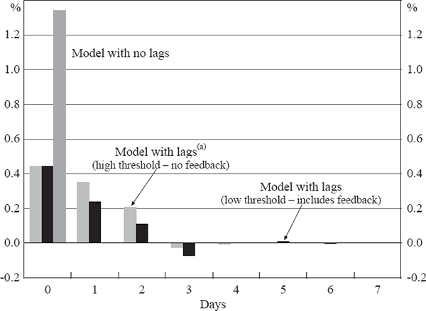
In the model with lags the coefficient on contemporaneous intervention does not measure the total impact of the intervention because there may continue to be changes in the exchange rate for several days. To quantify the impact of intervention it is useful to consider the impulse response function. An additional consideration in the model with lags is that an intervention shock can potentially lead to intervention on subsequent days, both because of the autoregressive and the exchange rate lags in the shadow intervention equation. Whether subsequent interventions occur will depend on the magnitude of the intervention thresholds. We consider two scenarios that bound the range of the exchange rate response. In the first, the intervention threshold is set so that there is no intervention on subsequent days. This is analogous to the traditional presentation of impulse response functions that map a one-time shock and so is comparable to the results in the model excluding lags. Secondly, we present impulse responses in which the threshold is effectively zero and so any non-zero shadow intervention is actually conducted.
Figure 6 shows these two impulse response functions along with the one for the base model without lags. Since the coefficients in the policy function on lagged interventions are negative, using a zero threshold for intervention implies that the central bank will partially unwind its intervention on subsequent days. Empirically this does not occur – the central bank almost never intervenes on opposite sides of the market on subsequent days. This highlights the importance of the interaction of the two components of the central bank policy function. The negative coefficients on lagged intervention result in a muted response of the exchange rate when the low threshold is used. Both scenarios demonstrate that the largest impact of intervention comes on the day it is conducted.
Note: (a) Restricts intervention equation so there is no intervention following the initial day
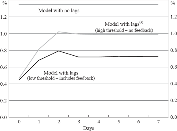
The cumulative impact of intervention is shown in Figure 7. Note that the short lag structure used implies that intervention has a permanent effect on the exchange rate. A long lag structure would be needed to capture the unwinding of the effects of intervention. Including many lags is not practical for the estimation method we employ and so we are unable to assess how long the effects of intervention last beyond a few days. The cumulative response of the exchange rate to intervention, after two to three days, is similar for the models including and excluding lags. In the model with lags A$100 million (US$100 million) will appreciate the exchange rate by 1 per cent (1.3 per cent), slightly less than the 1.4 per cent (1.8 per cent) predicted by the model excluding lags.
Note: (a) Restricts intervention equation so there is no intervention following the initial day
5.3 Caveats and Further Research
Before concluding, it is worth spending time discussing several caveats that should be addressed in future research. First, our estimation methodology does not distinguish through which channel intervention affects the exchange rate. Given the relative shifts in bonds in private hands is small, the portfolio balance channel is likely to play an insignificant role. Rather, the signalling channel, and possibly market microstructure effects, would seem to be responsible – but this is a conjecture, rather than a result.
Second, as it stands our methodology requires that the change in policy is truly exogenous. Finding such exogenous changes in policy for other countries may not be straight forward. However, it is possible to model the threshold in the participation equation as a function of macro variables, the exchange rate, and even the second moments of the endogenous variables. The procedure of estimation would be exactly the same as the one described here if the change in policy is thought of as a shift in the coefficients in that equation. Furthermore, the participation decision could be rationalised as a switching Markov regime where the transition probabilities are functions of the endogenous variables. The estimation of these models is beyond the scope of the present paper and is left for future research. Nevertheless, it is important to mention that in this paper we have emphasised the identification issue, and our specification is a reduced form representation of these models where the shift in policy would be reflected in changes in the intervention decision equation.
Finally, our methodology assumes that the coefficients, other than the threshold, are stable across regimes. This seems to be a reasonable assumption in the current study but may be more difficult to justify in other contexts. This criticism is akin to the application of the Lucas critique to models of monetary policy. Our framework is not entirely exempt from this critique, and therefore, conclusions from this analysis are subject to the caveat of the strength of these assumptions.
Footnote
If there are no lags in the system, the OLS estimate will be  .
[16]
