RDP 2003-03: Australia's Medium-Run Exchange Rate: A Macroeconomic Balance Approach 2. Modelling Macroeconomic Balance
March 2003
- Download the Paper 218KB
Williamson (1983) adopted the macroeconomic balance approach to derive estimates of exchange rates consistent with internal and external balance, which he labelled ‘fundamental equilibrium exchange rates’. This concept has sometimes been described as a current account theory of exchange rate determination, however, Wren-Lewis describes it as not a theory, but:
…a method of calculation of a real exchange rate which is consistent with [macroeconomic balance]. (Wren-Lewis 1992, p 75)
The approach is rooted in the balance-of-payments identity:

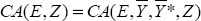
The right-hand side of Equation (1) is the current account CA which consists of the trade balance, net foreign income flows and net transfers. For Australia, most of the volatility in the current account is driven by changes in the trade balance. The current account balance in Equation (1) depends explicitly on the real exchange rate (E·P/P*), which affects the trade balance via the prices and volumes of imports and exports and that part of net foreign investment income that is denominated in foreign currency. It also depends on levels of domestic and foreign incomes, Y and Y*, as well as a variety of other factors Z that may shift the current account balance over time. The capital account is equal to the current account by definition.
2.1 Internal and External Balance
The macroeconomic balance approach rests on two concepts: internal balance and external balance.
The economies are in internal balance when output is at potential and current exchange rate effects have worked themselves through the system; that is, pass-through is complete. Both conditions reflect the medium-run nature of the concept. We define the current account consistent with these conditions as the ‘underlying current account’. In order to evaluate the underlying current account, the long-run elasticities of the current account with respect to the exchange rate and output have to be estimated. Internal balance is then reached when output is set to trend output. The exchange rate elasticity of the current account is needed to assess how much the current exchange rate has to move in order to bring the underlying current account to the target level.
External balance is achieved when the underlying current account is equal to the value of the target capital account, which is characterised as the sustainable desired net flow of resources between countries when they are in internal balance. The capital account is identically equal to the excess of domestic savings over investment. Therefore, Isard and Faruqee (1998) and Isard et al (2001) explicitly model the target capital account dependent on factors that influence optimal savings and investment decisions. Amongst others, these factors are the consumption smoothing decisions of the agents (i.e., the savings ratio), demographics (i.e., the dependency ratio), the relative fiscal position and capital needs determined by the development stage.
The macroeconomic balance approach models exchange rate equilibrium as the level that generates an underlying current account equal to the target capital account when the domestic and foreign economies are in internal equilibrium.
It should be noted that this approach is based on a medium-term equilibrium which is likely to change over time. One reason is that the factors determining the target capital account, such as demographics or fiscal policy, can change over time, which would imply a corresponding change in the exchange rate. Another reason is that the underlying current account for a country might change both over time and relative to other countries. We treat only changes in output (relative to potential) and the exchange rate as endogenous to our model. Any change in an exogenous variable can therefore change the underlying current account (some examples are discussed in Section 2.3). This implies that the value of the equilibrium exchange rate will depend on the time period in which it is calculated.
2.2 The Macroeconomic Balance Approach in Three Steps
The macroeconomic balance approach can be implemented in three steps:
- Choose a sustainable, or target, capital account KAtarget.
-
Derive the underlying current account
 where
where  and
and
 are
potential outputs and Z is a set of other exogenous variables.
are
potential outputs and Z is a set of other exogenous variables.
- For each assumed value of KAtarget, solve for the exchange rate that satisfies KAtarget = CA(E,Z).
Step 1: The target capital account
The target capital account is usually arrived at judgementally, taking positions on optimal savings and investment decisions. Often it is taken as the medium-run average of the actual current account. Or it is explicitly modelled as in Isard et al (2001) and Williamson and Mahar (1998). However, in this paper we avoid modelling the target capital account and instead provide a range of estimates of equilibrium exchange rates associated with alternative assumptions about the capital account position.
Step 2: The underlying current account
Since we take an agnostic view on the target capital account, we can move straight to Step 2. We decompose the current account into trade balance (X-M), net foreign income NID[3] (which consist mainly of net investment income arising from interest, profit and dividends), and net transfers NT. We model these three building blocks separately to identify the elasticities of each component to changes in the exchange rate and to output.

The second and third component of the current account, net investment income and net transfers are modelled in the simple way suggested by Wren-Lewis and Driver (1998), henceforth WD. Investment income derived from assets denominated in foreign currency will move directly with the exchange rate. Net transfers are assumed to be independent of demand or the exchange rate.
The first component, the trade balance, is the heart of the underlying current account equation and requires more modelling effort. The focus of our study is very similar to that of WD, in that they concentrate on estimating the price and income elasticities of the trade flows that underlie the trade balance. We expect exports to increase if the exchange rate E depreciates or if world demand increases. Imports will increase with domestic demand or when the exchange rate appreciates. The trade balance will thus increase when the domestic currency depreciates. So much for the theory. Goldstein and Khan (1985) have shown that estimated trade elasticities often turn out to be effectively zero. Or worse, they might have the wrong sign. In practice, therefore, elasticities are often imposed for some equations, as for example in WD or Isard et al (2001).
Once we have estimated all trade elasticities we can use them in Equation (2) to model the underlying current account as a function of the exchange rate E. We evaluate this function after setting domestic and foreign output to their trend levels and setting all exogenous variables to their actual values at specific dates.
To make useful comparisons over time and between countries, the current account is usually modelled as a proportion of nominal GDP, P-Y. Equation (2) then becomes:

Step 3: Solving for the exchange rate
Step 3 is straightforward. Once Equation (3) is estimated and output gaps are set to zero, it is then possible to calculate the level of the exchange rate E which equates CA(E) with the target capital account. Figure 1 summarises the relationship between the equilibrium exchange rate and the assumed capital account position: E* would be the equilibrium which corresponds to the target KA.
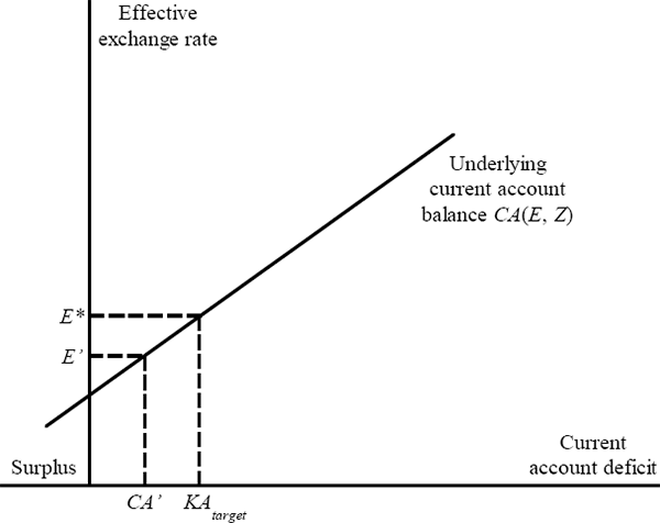
Source: Isard and Faruqee (1998)
If the exchange rate was E', Step 2 would identify CA' as the underlying current account position. CA' will be different from the observed current account to the extent that output gaps are not zero. Step 3 would then tell us how much the exchange rate has to change to equilibrate the underlying current account with the target KA. The necessary change is broadly the difference between E' and E*.
2.3 Limitations of the Macroeconomic Balance Approach
The macroeconomic approach has – like every concept of calculating equilibrium exchange rates – a number of shortcomings.
Some limitations relate to the implementation of the approach. Firstly, judgement is necessary to decide on the target capital account. Secondly, some trade elasticities are notoriously difficult to estimate, and low exchange rate elasticities of the trade balance may imply implausibly high estimates of the sensitivity of the equilibrium exchange rate to the assumed capital account position.
A more conceptual problem is that the underlying current account, and therefore the equilibrium exchange rate, might change over time as a result of changes in other variables that determine Equation (3).[4] WD distinguish four sources of such changes. First, there may be a trend in some components of trade, such as a declining (world) export share. Second, trend rates of GDP growth at home and abroad might differ. This can imply a different rate of change for exports and imports, and thus a change in the trade balance. Third, estimated income elasticities may be different for exports and imports. Then, even if domestic output grows at the same trend rate as foreign output, the trade balance (and therefore the underlying current account) would change. Fourth, the approach does not impose a stock equilibrium. A non-zero current account target implies a continuing change in the net foreign asset position. For instance, a country that runs an underlying current account deficit lowers debt interest receipts and further increases the current account deficit (the reverse holds for a country in surplus). This would require a trend depreciation unless GDP grows at the same rate as the net foreign asset position.
Finally, the approach does not explain the dynamics of the adjustment to the macroeconomic balance exchange rate. Taking the functional relationship in Equation (1) literally would imply a causal relationship from the target capital account to the exchange rate. However, as discussed earlier, the macroeconomic balance methodology involves calculating an exchange rate that is consistent with internal and external equilibrium – it is silent about the dynamics of the adjustment. The exchange rate is merely the relative price that facilitates the adjustment of the underlying current account to the target capital account.
Footnotes
Note that the net foreign investment income in Australia is usually shown as a deficit number. Therefore we have to subtract the NID term in Equation (2). [3]
There are two ways to address this problem. WD make their estimates period-specific and calculate them for different years. Isard and Faruqee (1998) account for the ‘drift’ due to changes in non-modelled variables by correcting the intercept of the trend current account in each period. [4]