RDP 2003-03: Australia's Medium-Run Exchange Rate: A Macroeconomic Balance Approach Appendix B: Estimation Results

In this appendix we describe the estimated equations of the current account components. All lower-case variables are in logs. For illustration purposes we only report the long-run coefficients of the VECM estimates. The estimated equations show the point estimates with the standard errors (where available) in brackets.

Agricultural Exports

This is described in the main text.

Resource Exports

We assume that Australian producers of resources are price takers, therefore we are left with estimating the supply curve. Resource export supply is a function of real unit labour costs and the level of real GDP, which capture capacity constraints and factor costs. A significant price effect with the correct sign could not be detected.

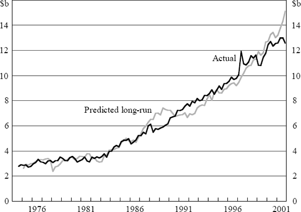
We estimate the long-run relationship below using a VECM with eight lags. Figure B1 shows how our long-run model compares with the actual series.

where x_res is the volume of resource exports, p_lab are real unit labour costs, and y is Australian real GDP.

Manufactured Exports

This is described in the main text.

Service Exports

For service exports we assume Australian producers are price setters. This allows us to concentrate on estimating the demand curve only. Demand for service exports is modelled as a function of relative prices and world income.

We estimate the long-run relationship below using a VECM with eight lags.

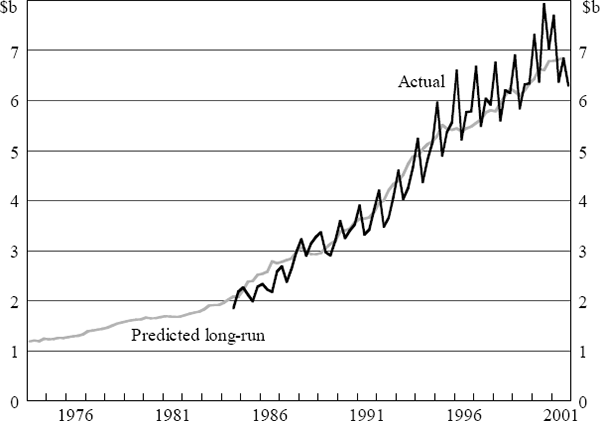
where x_srv is the volume of exported services, is the world CPI, e^twi is the effective exchange rate, p_cpi is Australian CPI, and y^world is world real GDP. The result is illustrated in Figure B2.

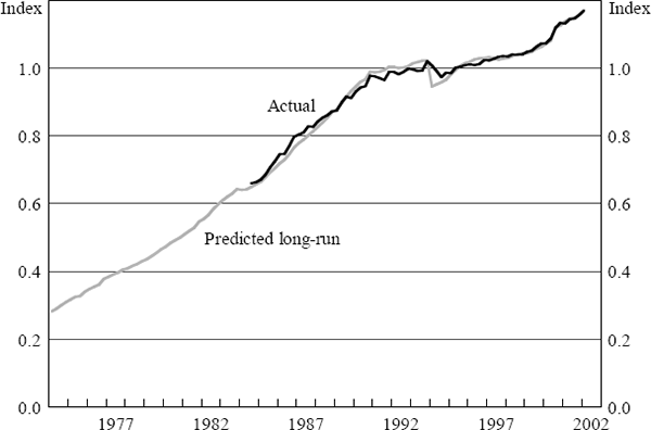
The price setting assumption is worth an additional comment. We assume that the Australian price of service exports is determined by the Australian CPI. However, a level shift is apparent from 1994 in the service exports price deflator (see Figure B3), caused by a drop in the price deflator of two of the five subcategories of service exports. The change in the way these series are measured is responsible for the sudden level shift.^[16] We include in our model of export service prices a dummy variable to capture this change. Note that the regression is in levels, rather than logs.

where is the Australian price of exported services, P_cpi are Australian consumer prices, D1 = 1 in all time periods before 1994:Q1, and D1 = 0 in all time periods including and following 1994:Q1.

Initially we estimated this equation using unrestricted OLS and used these results to test the hypothesis that the coefficient on P_cpi was unity, which was accepted (p-value in excess of 0.55). This confirms that our assumption of price setting is reasonable. We therefore imposed this restriction for the estimation results presented in Equation (B3).

Goods Imports

For imported goods we allow for full pass-through, which allows us to identify a demand function. Demand is modelled as a function of relative prices and domestic income.

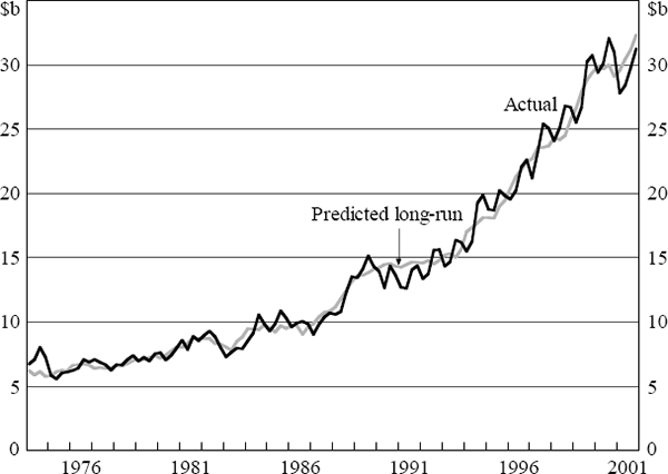
We estimate the long-run relationship below using a VECM with four lags.^[17]

where m_gds is the volume of imported goods, is the world price of export goods, e^twi is the effective exchange rate, p_ppi is the Australian PPI, and y is Australian GDP.

Service Imports

It proved to be very difficult to find a model of service imports. Estimates were highly dependent upon the technique and the dynamic structure chosen. The impact of the exchange rate was difficult to gauge. It appeared to have a significant impact on volumes but with the wrong sign. For prices, there was very low pass-through of exchange rate changes. We obtained exchange rate elasticities by combining regression analysis (with economic priors imposed) and personal communication with the ABS.^[18]

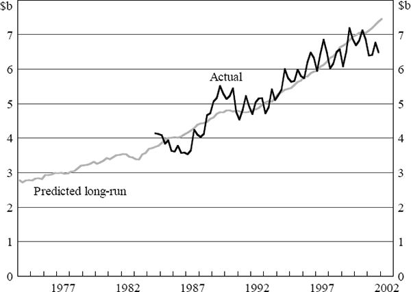
For volumes (Figure B5), we imposed a zero exchange rate effect, and estimated a long-run relationship using a VECM with three lags.

where m_srv is the volume of imported services and y is Australian GDP.

For prices, we explain the Australian dollar price of imported services as a function of the world CPI and the exchange rate, using the following equation.

where is the Australian price of imported services, are world consumer prices, and e^twi is the effective exchange rate.

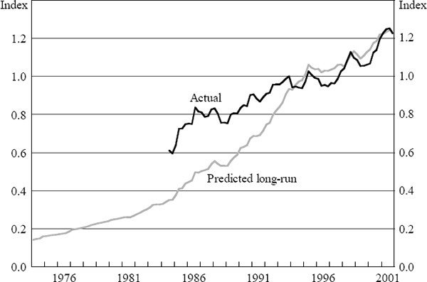
Initial estimates of this equation gave a pass-through well below unity (0.2). Upon consultation with the ABS, we decided to impose an exchange rate elasticity of 0.5.^[19] In our preferred model, we imposed the elasticity and used OLS to estimate the constant. This model predicts quite well from the mid 1990s as can be seen in Figure B6.

Net Income Deficit (NID)

The net income deficit is the difference between income credits (payments accruing to foreign assets) and income debits (payments accruing to foreign liabilities).^[20] Since we only incorporate the valuation effects arising from changes in the exchange rate, income credits and debits need not be estimated. Here all variables are in levels.

where α₁ denotes the proportion of foreign assets denominated in foreign currency (in our case US$), A is the stock of foreign assets (equity + debt) in Australian dollars, e^twi is the effective exchange rate, and r^A is the implied interest rate on foreign assets.

where α₂ denotes the proportion of foreign liabilities denominated in foreign currency, D is the stock of foreign liabilities (equity + debt) in Australian dollars, e^twi is the effective exchange rate, and r^D is the implied interest rate on foreign liabilities.

The share of assets and liabilities denominated in US$ is the actual share in the reference period, for which the equilibrium exchange rate is evaluated. For the June quarter 2000, we calculate that α₁ = 0.91 and α₂ = 0.36.^[21] That implies that while most foreign assets are denominated in foreign currency, most foreign liabilities are denominated in Australian dollars. Although net foreign liabilities are positive, and equal to roughly 60 per cent of GDP, net foreign liabilities denominated in foreign currency are actually (slightly) negative. This has the surprising implication that a depreciation fails to increase net income outflows.^[22]

Transfers

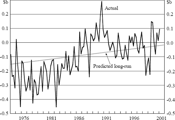
Net transfers are modelled using a simple linear time trend. All variables are levels. The coefficients are estimated using OLS.

where NT are net transfers (in Australian dollars) and t is a time trend. The estimated trendline is show in Figure B7.

Footnotes

From December quarter 1994, these two subcategories (‘transportation services’ and ‘passenger and other services’) are linked to the CPI for international airfares whereas prior to that quarter they are calculated as the total revenue earned from abroad and home divided by the number of arrivals and departures (personal communication with the ABS). [16]

It was difficult to choose between a VECM with four versus five lags. We chose the former because the data is quarterly. With five lags, the elasticity was 0.72 compared to 0.67 with four lags (this is rounded to 0.7 in Table C3). [17]

Ideally, one would estimate a reduced form as in the case of manufactured exports. However, the estimated coefficients in such a model are not theoretically consistent (the income and price elasticities both have the wrong sign), whereas the model we use gives theoretically consistent results. [18]

In a typical year, service imports are split evenly three ways between transport (half being sea freight and half being passenger air travel), travel (service imports for tourists, such as haircuts) and other services (business services, royalties, communications, accounting services, embassy expenditures etc). With regard to the exchange rate effect on transport prices, significant oversupply exists in container shipping and passenger air travel, so it may be the case that carriers are pricing to market. However, one would expect much of the travel is priced in overseas currency, as is a sizable proportion of other services (personal communication with the ABS). As a rough guess, we decided that about half of service imports could have full exchange rate pass-through. [19]

Compensation from foreign employment is a third component. However, this is negligible in size, and we have therefore excluded it from our analysis. [20]

We use an internal data source which corresponds to that in ABS Cat No 5352.0. These data are subject to frequent revisions. The figures are current as at June 2002. [21]

Not surprisingly, both income credits and income debits fitted the data well, since the model has the US$ levels of each available in the simulation. [22]