RDP 1999-04: Value at Risk: On the Stability and Forecasting of the Variance-Covariance Matrix 3. Models for Forecasting the Variance-covariance Matrix

The apparent instability of the unconditional covariance matrix suggests that the historical covariance approach will be an inaccurate estimator of the true variance-covariance matrix. Therefore, more complex models of the evolution of the variance-covariance matrix may be required when forecasting risk exposures.

The three classes of models that we investigate are the equally weighted historical approach, the exponentially weighted moving average approach and the GARCH approach. There are many other types of models that may be used. We have, however, restricted ourselves to those models (and simple variations of those models) that are currently used by Australian banks.

The previous section's stability testing was based on standard covariance and correlation measures which take account of each series' sample mean over each sub-period. In the analysis that follows it is assumed that each financial return series has a zero mean. This assumption is a commonly used market practice when measuring market risk exposures. From a theoretical perspective the mean is both close to zero and prone to estimation error; thus, estimates of the variance-covariance matrix may be made worse by the inclusion of an inaccurate estimate of the mean (see Figlewski (1994)). If the standard formula for the variances and covariances is considered the squared return component is of the order 100 to 1,000 times greater than the mean component, hence, the inclusion of the estimate of the means will not make a significant difference.

While several banks, in their implementation of a VaR model, re-estimate the variance-covariance matrix daily, it is common practice in other banks to update the variance-covariance matrix only once a quarter. As a result we consider two sets of forecasts: the one-day-ahead forecasts and the forecast average variances and covariances over the quarter ahead.

3.1 Fixed-weight Historical

The fixed-weight approach assumes that return covariances and variances are constant over the sample period. Our finding of instability in the variance-covariance matrix indicates that this is not a good assumption. However, it is widely used on simplicity grounds. Using this approach, each element in the variance-covariance matrix can be represented by:

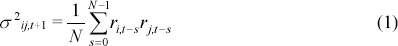
where r_i,t−s represents the market return for asset i between days t−s−1 and t−s.

3.2 Exponential Smoothing

Rather than placing equal weight on past observations, exponential smoothing places more weight on the most recent. This approach was popularised by JP Morgan in their RiskMetrics VaR model (JP Morgan and Reuters, 1996). The exponentially weighted moving average approach reacts faster to short-term movements in variances and covariances. If the underlying variances and covariances are not constant through time this faster reaction is an advantage. On the other hand, giving a greater weight to recent data effectively reduces the overall sample size, increasing the possibility of measurement error. Each element of the variance-covariance matrix is represented by:

where 0<λ<1

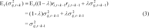
An exponentially weighted average on any given day is a combination of two components: yesterday's weighted average, with weight λ, and yesterday's product of returns, which receives a weight of (1−λ). This equation incorporates an autoregressive structure for the variance-covariance, thus reflecting the concept of volatility clustering. In the subsequent analysis two approaches are implemented. The first is to assume, consistent with the RiskMetrics specification, that λ is constant at 0.94. The second approach is to estimate λ over successive rolling windows using maximum likelihood techniques (we shall refer to this approach as the dynamic exponentially weighted moving average approach).

To gauge the accuracy of fixing λ at 0.94, the model is estimated using maximum likelihood methods over the full sample (λ was constrained to take the same value for all elements of the matrix). The value obtained from this analysis using the foreign exchange covariance matrix is 0.995.^[3]

Like the equally weighted method the k-step ahead one-day forecasts are constant and the quarter-average forecast is equal to . To see this:

3.3 Multivariate GARCH

The GARCH model of Bollerslev (1986) is a generalisation of the ARCH model introduced by Engle (1982). Variances and covariances are specified as stochastic processes that evolve over time. The intuition behind these models is similar to the exponentially weighted approach in that volatility clustering may be explicitly modelled. Less restrictions, however, are placed on the specification of the volatilities' behaviour. The previous two models are nested within the GARCH model. If α and β are zero in the below specification then the model collapses to the fixed-weight historical model. If ω is equal to zero, α = (1−λ) and β = λ then the model is equivalent to the exponentially weighted model. In a univariate setting the zero-mean GARCH(1,1)^[4] model has the form:

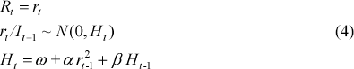
The vector of innovations or unexpected returns is assumed to be conditionally normal with a conditional variance of H_t. The multivariate framework is analogous to the univariate in that the variance-covariance matrix is conditioned on past realisations of covariances of financial returns but the specification of the evolution of the covariances can become more complicated.

The more general multivariate models assume that variances and covariances rely on their own past values and innovations as well as other variables' past values and innovations. The number of parameters to be estimated in these general models is such that, as the number of variables increases, computation can become intractable. To illustrate, for our nine-by-nine foreign exchange matrix the number of parameters to be estimated by one of the more general models is 243. Given that our focus is on a model's forecasting performance, which requires repeated rolling estimation of the models, a more parsimonious parameterisation is needed.

To this end two models are used. The first model is the constant correlation multivariate GARCH model developed by Bollerslev (1990). The model has the advantage of reducing the number of parameters to be estimated to 3p + p(p−1)/2 where p is the number of financial returns. Variances are estimated using a simple GARCH(1,1) formulation:

The covariances are formulated as:

Non-negativity constraints need to be imposed on the variance parameters to ensure that the conditional variance estimates are always positive. Given the recursive nature of the system, stationarity requires that α_i + β_i < 1 for all i.

The parameters of the model are estimated by maximum likelihood techniques. Under standard regularity conditions the maximum likelihood estimator is asymptotically normal.^[5] The log-likelihood is maximised using the Bernt, Hall, Hall and Hausman (1974) algorithm. Given the highly non-linear structure of the log-likelihood the iteration process is extremely time intensive. Even after the constant correlation assumption is imposed on the model the 63 parameters in the full system (for the nine-by-nine foreign exchange variance-covariance matrix) make rolling estimation computationally intractable. To facilitate rolling estimation the approach taken is to estimate separate bivariate systems for each pair of financial returns. Each of these 36 systems have seven parameters to be estimated. From these bivariate systems the full variance-covariance matrix can be constructed. To the extent that covariances are in fact jointly determined estimates produced from the pair-wise estimation may be biased and inefficient. Also, this approach can not guarantee positive defmiteness of the covariance matrix but does enable forecasts to be constructed in a tractable fashion. This approach provides only one estimate of each covariance, but ρ−1 estimates for the ω, α and β parameters for each variance. The average of the ρ−1 forecasts of each variance is used.

The one-day-ahead GARCH variance forecast for the constant correlation GARCH model is given by:

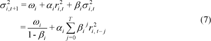
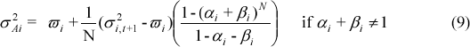
T represents the length of data used in the estimation. It follows that the k-step ahead forecast has the form:

and hence, are not constant in k. Given these variance forecast functions the average one-day forecast over a quarter (containing N days) is:

The covariance forecasts are simple functions of these variance forecasts and the parameters ρ_ij given the constant correlation assumption.

This constant conditional correlation specification has been used widely in the literature to facilitate estimation given the difficulty in estimating multivariate GARCH models, but its validity is open to debate. The assumption could be justified if the conditional correlation remains constant over time but the market expected returns and variances vary over time. There is evidence of predictable time variations in the equity return distributions; the variance of returns has been shown to be heteroscedastic and univariate GARCH models have had success in modelling returns' variances (see Alexander and Leigh (1997) and Figlewski (1994)). Factors which weigh against the constant correlation assumption include the increased interdependence of international markets (growing integration could lead to increasing correlations through time); the fact that markets tend to be more strongly correlated in times of high volatility than in times of low volatility and the results of our own stability testing discussed previously. Appendix B analyses deviations from the simple constant correlation model. The results imply that this assumption of a constant conditional correlation is questionable; threshold and time-trend models are able to explain movements in conditional correlations. In the following forecasting exercise the results from this analysis should be taken into account. Poor forecasting performance of the constant conditional GARCH model may be due to mis-specification of the model.

The second multivariate GARCH model that we use for forecasting is the Babba, Engle, Kraft and Kroner (BEKK) parameterisation. Engle and Kroner (1995) introduced this model because its quadratic form guarantees that the conditional covariance matrix will be positive definite. The model has the form:

Matrices A, B and C are the parameter matrices that need to be estimated. R_t is a vector of returns for time t. H_t is the estimated variance-covariance matrix at time t. Again the unconstrained BEKK model is too computationally time consuming for use in this forecasting exercise. To facilitate tractability, a diagonal structure is imposed on the parameter matrices, which removes cross market influences. The model automatically imposes the necessary non-negativity constraints. Rather than producing estimates pair-by-pair, the full model is estimated. Variance forecasts from the BEKK model have the same form as those from the GARCH constant correlation model, with the GARCH parameters being replaced by squared parameters. The covariance forecasts in the BEKK model relax the constant correlation assumption and have the same specification as the constant correlation GARCH variance equations.

Footnotes

This is not statistically significantly different from 0.94. [3]

The (1,1) denotes one lagged variance term and one lagged squared return. [4]

Following Bollerslev (1986), if the model correctly specifies the first two conditional moments but the conditional normality assumption is violated, under suitable regularity conditions the quasi-maximum likelihood estimates will be consistent and asymptotically normal, but the usual standard errors have to be modified. [5]