RDP 9801: Labour Market Adjustment: Evidence on Interstate Labour Mobility 4. Tests of Labour Mobility
February 1998
- Download the Paper 314KB
In this section of the paper, we examine how variation in labour market performance across states has been affected by labour mobility. We present the results of three simple tests of the role of mobility in labour market adjustment. First of all we present some facts about interstate migration.
Total interstate migration activity can be examined by considering gross flows data (gross flows are defined as the sum of in- and out-migration for a state). By this measure, migration flows have increased somewhat; gross flows as a share of population have risen from 3.3 per cent in 1976 to 4.0 per cent in 1996, an increase of 18 per cent.[7] This result is consistent with the view that economic integration between Australian regions has increased over time.
Another perspective on labour mobility can be obtained by examining data from the ABS Survey Australians' Employment and Unemployment Patterns (ABS Cat. No. 6286.0). Table 1 shows the response of job seekers to the question ‘Would you be prepared to move interstate if offered a suitable job?’
| State | Percentage | State | Percentage |
|---|---|---|---|
| New South Wales | 31.4 | Western Australia | 34.2 |
| Victoria | 36.9 | Tasmania | 41.2 |
| Queensland | 34.1 | Northern Territory | 50.0 |
| South Australia | 43.1 | ACT | 48.2 |
In general, respondents in states with relatively poorly performing labour markets (particularly South Australia and Tasmania) are more receptive to moving interstate to find employment. This result supports the view that labour migration does respond to state labour market conditions. Respondents in smaller states are generally more willing to move interstate, possibly because the breadth and diversity of job opportunities is less in smaller states.
The above survey question assumes that the respondent has been offered a job in another state with certainty. If employment in the new state is not guaranteed, two further impediments to mobility exist, in addition to the costs of migration discussed in Section 2 in terms of the Harris-Todaro model. Firstly, individuals may have inadequate or misleading information about relative job opportunities in different states. Secondly, prospective interstate migrants have limited access to local job networks in other states, reducing their probability of employment interstate. Both these factors act to reduce the incentive for an individual to migrate.
Table 2 details migration levels for each state and territory for the year ended 30 June 1996. Note that the table only reflects internal flows within Australia, not flows to and from other countries.
| State | Arrivals | Departure | Net migration | Net migration/ population (per cent) |
|---|---|---|---|---|
| (000s) | (000s) | (000s) | ||
| New South Wales | 87.9 | 103.5 | −15.7 | −0.25 |
| Victoria | 57.1 | 73.4 | −16.4 | −0.36 |
| Queensland | 113.5 | 76.0 | 37.5 | 1.12 |
| South Australia | 25.9 | 32.1 | −6.2 | −0.42 |
| Western Australia | 33.2 | 29.4 | 3.8 | 0.22 |
| Tasmania | 10.6 | 13.3 | −2.7 | −0.58 |
| Northern Territory | 18.9 | 18.7 | 0.1 | 0.07 |
| ACT | 19.0 | 19.5 | −0.5 | −0.15 |
Three states experienced positive net migration flows: Queensland, Western Australia and the Northern Territory. Of these, flows to Queensland were by far the largest. In fact, interstate migration to Queensland was large enough to absorb the net out-migration from New South Wales, Victoria and South Australia. Tasmania and South Australia experienced the largest net out-migration relative to population. Both these states lost about half of 1 per cent of population through interstate migration over 1995/96.
Thus, the two states with the lowest employment growth have the highest out-migration, and the two with strongest employment growth have the highest in-migration. This evidence is consistent with the view that workers migrate in response to labour market differentials between states. However, this conclusion should be treated cautiously, since the direction of causality between labour migration and employment growth is unclear.
If labour was perfectly mobile across the states, we might expect all the states to have the same unemployment rate in the longer term. In practice, however, there might be persistent differences in state unemployment rates, because of compensating differentials in wages, lifestyle etc. One simple test of the role of labour mobility as an equilibrating mechanism, is to examine whether the state unemployment rates are cointegrated with the national rate.[8] In conducting this test, we allow for a constant difference between a state's unemployment rate and the national rate.
The results of the cointegration tests show that the null hypothesis of no cointegration can be rejected for South Australia, Tasmania and the two territories, suggesting some degree of labour mobility (Appendix A). In contrast, Groenewold (1992) finds that state unemployment rates have no tendency to converge to a common national rate, even in the long run. Note however, that our test for cointegration does not impose a common unemployment rate because we allow for constant terms in the cointegrating relations.
We also estimate a VAR of the state unemployment rates and test for cointegrating relations between the states using the Johansen (1988) procedure. If labour market adjustment acts to close unemployment-rate differentials between states over time, then there should be seven cointegrating relations between the eight states and territories. Results of this test are also presented in Appendix A. Two cointegrating relations were found between the eight state unemployment rates. To better identify the nature of the cointegrating vectors, a series of exclusion restrictions was tested but each of these restrictions was rejected at the 5 per cent level.
These results suggest that labour market adjustment does act to decrease unemployment differentials between states over time, although a modelling strategy based on unemployment rates alone is not sufficient to capture the relevant adjustment mechanisms.
A second simple indicator of the degree of labour mobility is the standard deviation of the state unemployment rates. If labour was perfectly mobile we would expect that the standard deviation would be close to zero, as unemployment differentials would be quickly eliminated. Figure 5 shows that the standard deviation of the state unemployment rates has risen over time to around 1.5 per cent (the figure is just over 1 per cent if the territories are excluded from the calculation). This is only slightly higher than the dispersion of the state unemployment rates in the United States and considerably lower than the dispersion of regional unemployment rates for the European Community reported in Eichengreen (1990), suggesting that labour mobility in Australia may be similar to that in the US.
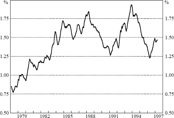
However, this measure of mobility is affected by the dispersion of shocks across the different states. If the states in the US have larger idiosyncratic shocks than in Australia (for example, because of greater differences in industry composition), in the short run, we would expect greater dispersion of unemployment rates in the US, regardless of the degree of labour mobility. On the other hand, there are larger distances between capital cities in Australia, and hence, greater costs of relocation, which may increase the persistence of state unemployment differentials.
Thirdly, we regress the ratio of net migration into a state to the state's population on the state's relative unemployment rate differential. Our prior is that a high state unemployment rate will encourage out-migration from that state, thus the coefficient on the unemployment rate differential should be negatively signed. We also regress the absolute value of the net migration ratio on the absolute value of the unemployment differential and the national unemployment rate. If individuals are liquidity constrained in times of high unemployment, then the magnitude of total migration flows might be expected to fall.
In both cases, a fixed-effects panel regression was conducted. The results are presented in Table 3.
| Regression 1: | ||||
|---|---|---|---|---|
 |
||||
| αNSW = −0.0041 | (−3.55) | αWA = 0.0023 | (1.98) |  = 0.34 = 0.34
|
| αVIC = −0.0056 | (−4.76) | αTAS = 0.0010 | (0.77) | |
| αQLD = 0.0156 | (13.97) | αACT = −0.0060 | (−4.74) | |
| αSA = −0.0000 | (−0.04) | αNT = −0.0011 | (−0.78) | |
| Regression 2: | ||||
 |
||||
| αNSW = 0.0090 | (5.08) | αWA = 0.0081 | (4.58) | = 0.41
|
| αVIC = 0.0092 | (5.21) | αTAS = 0.0089 | (5.00) | |
| αQLD = 0.0199 | (11.29) | αACT = −0.0217 | (12.06) | |
| αSA = 0.0074 | (4.23) | αNT = −0.0126 | (6.84) | |
Notes: t-statistics in parentheses |
||||
As expected, the higher a state's unemployment rate relative to the national rate, the more people leave (less people enter) the state. If a state's unemployment rate rises one percentage point above the national unemployment rate, there is a 0.25 percentage point increase in net out-migration relative to population. The state-specific constant terms are significant in most cases, indicating that some net interstate migration occurs even in the absence of interstate unemployment differentials. The migration/population rates have been annualised, thus a coefficient of 0.0165 (as for Queensland), implies an annual net migration/population ratio for that state of 1.65 per cent in the absence of unemployment differentials. The results in the second regression show that the higher the national unemployment rate, the less people migrate between states.
Collectively, the evidence from these three tests suggests mobility does play a significant role in labour market adjustment. In particular, the relatively low dispersion of state unemployment rates, and the significant influence of unemployment differentials on migration patterns supports the role of migration as an adjustment mechanism. However, in the case of Tasmania and South Australia, this mobility has been insufficient to reduce unemployment in those two states to the national average. In addition, the cointegration analysis provides somewhat ambiguous evidence of labour mobility as an adjustment mechanism to state-specific shocks. Since state unemployment rates are highly correlated with aggregate unemployment; and given that labour migration already appears to work reasonably well in moderating state labour market differentials, it is questionable whether higher mobility would greatly reduce the national unemployment rate.
Footnotes
Migration, Australia, ABS Cat. No. 3412.0. [7]
Clearly a precursor to undertaking this analysis is establishing that the state unemployment rates are actually non-stationary. A panel unit root test was conducted on the pooled state unemployment rates which concluded that it was not possible to reject the null hypothesis that the state unemployment rates were integrated of order 1 at the 5 per cent level of significance. [8]