RDP 9708: Measuring Traded Market Risk: Value-at-risk and Backtesting Techniques 3. Backtesting
November 1997
- Download the Paper 400KB
As the previous discussion has demonstrated, there is a range of methods in use for calculating VaR estimates. In practice, even where banks use the same broad methods to calculate VaR, there is considerable variation in the application of those VaR methodologies – different models may be used to measure the sensitivities of particular instruments to price movements (particularly for options and other more complex products; see, for example, Cooper and Weston (1995)); different methods may be used to aggregate exposures across instruments; and different techniques for estimating price volatilities may be used.
Since there is such a divergence in the VaR methodologies and their application across banks, and given the debate about the veracity of the statistical assumptions underlying VaR calculations, it is useful to test the performance of VaR models. Such testing is often referred to as ‘backtesting’.
Many banks that use VaR models routinely perform simple comparisons of daily profits and losses with model-generated risk measures to gauge the accuracy of their risk measurement systems. However, banks themselves are only just beginning to develop more sophisticated backtesting techniques and there are considerable differences in the types of tests performed.
In this paper we consider the following tests of VaR model performance:
- the regulatory backtest required as part of the capital-adequacy framework;
- exceptions testing which examines the frequency with which losses greater than the VaR estimate are observed;
- variance testing which compares the estimate of profit and loss variance implicit in a VaR estimate with the realised variability of profits and losses over time;
- tests to assess whether the profit and loss data are normally distributed; and
- a risk-tracking test evaluating the correlation between VaR estimates and the magnitude of daily profit and loss results.
To illustrate these tests we apply each of the tests to VaR and profit and loss data for a number of individual trading portfolios obtained from an Australian bank.
3.1 Shortcomings of Backtesting
Before presenting the tests themselves we note that there are a number of difficulties with the general approach to backtesting which uses realised profit and loss results. The most fundamental of these arises from the fact that such backtesting attempts to compare static portfolio risk with a more dynamic revenue flow. VaR is measured as the potential change in value of a static portfolio, at a specific point in time (typically end-of-day). Hence, the VaR calculation assumes that there is no change in the portfolio during the holding period; the portfolio can be viewed as representing a stock of risk at a given point in time. In practice, banks' portfolios are rarely static, but change frequently. Profits and losses are flows accruing over time as a bank takes on and closes out positions reflecting changes in portfolio composition during the holding period.
The difficulties that dynamic portfolios create can be illustrated most starkly by considering a trading desk that is not permitted to hold open positions overnight. During the day the desk may take positions and as a result experience large swings in profit and loss, but at the end of each day all positions must be closed out. Hence, an end-of-day VaR will always report a zero risk estimate, implying zero profit and loss volatility, regardless of the positions taken on during the day. More generally, where open positions remain at the end of the trading day, intra-day trading will tend to increase the volatility of trading outcomes, and may result in VaR figures underestimating the true risk embedded in any given portfolio.
To overcome this problem of dynamic portfolios, a backtest could be based on a comparison of VaR (using a one-day holding period) against the hypothetical changes in portfolio value that would occur if end-of-day positions were to remain unchanged. That is, instead of looking at the current day's actual profit or loss, the profit or loss obtained from applying the day's price movements to the previous day's end-of-day portfolio is calculated (this is often referred to as ‘close-to-close’ profit and loss). This hypothetical profit or loss result could then be compared to the VaR based on the same, static, end-of-day portfolio. In such a case, the risk estimate and the profit and loss would directly correspond. At this stage, several Australian banks do perform analysis on this basis.
The distortion in backtesting comparisons arising from changes in portfolio composition can be minimised by selecting a shorter holding period. Clearly movements in portfolio composition will be greater the longer the chosen holding period. It is for this reason that the Basle Committee recommends that backtesting be conducted based on a one-day holding period even though the capital that a bank is required to hold against its market risk is based on a VaR with a ten-day holding period (Basle Committee on Banking Supervision 1996a).
Further difficulties in conducting backtests arise because the realised profit and loss figures produced by banks typically include fee income and other income not attributable to position taking. While identification of fee income is relatively straightforward, isolating profits generated solely from position taking may be more difficult. Acting as a market maker allows banks to earn profits by setting different bid and offer rates; even transactions conducted with a view to profiting from market movements may profit from the bid/offer spread. A more sophisticated approach to measuring profitability would involve a detailed attribution of income by source, including fees, spreads, market movements and intra-day trading results. In such a case, the VaR results should be compared with the income generated by market movements alone. While most Australian banks do separate fee income from trading profit and loss, more refined attribution of income focusing on isolating revenue derived from position taking is generally only done in limited cases (for example, where proprietary trading is conducted by traders separate from those involved in other trading activity).
It may be argued that fee income and other market-making income are an inherent part of a bank's business and hence, their variability should be taken into account when assessing the riskiness of the bank's trading operations and when evaluating the performance of risk-measurement techniques. However, the VaR models in use at most banks are designed to measure outright position risk rather than risk arising from volatility in fee income or from movements in bid/offer spreads which may require the use of other modelling techniques. Thus the objective of backtesting should be to compare measured position taking risk with pure position taking revenue.
It should be kept in mind that shortcomings in the construction and practical implementation of a VaR model may not be the only reason why models fail backtests. As discussed in Section 2.7, VaR models do have some fundamental shortcomings. A VaR model is reliant on historical data and cannot capture major regime shifts in markets. Large swings in intra-day trading or an unusual event in trading income other than from position changes can lead to poor outcomes not reflective of the quality of the VaR model's construction.
3.2 The Sample Portfolios
The following sections step away from the data issues discussed above and look at some of the tests currently in use in banks in Australia and overseas. Those tests are applied to daily VaR and realised profit and loss data obtained from an Australian bank; the data cover the period from January 1992 to February 1995. The bank uses the variance-covariance approach to calculate a one-day holding period VaR.
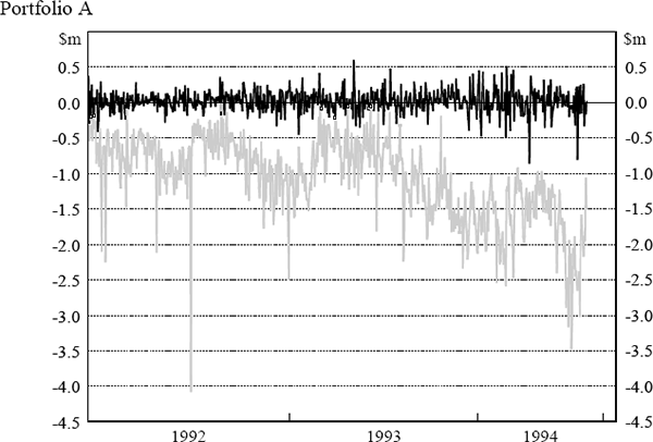
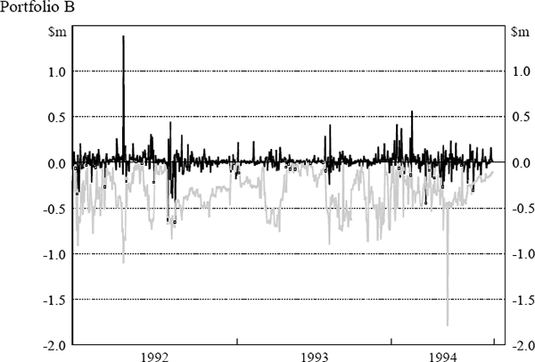
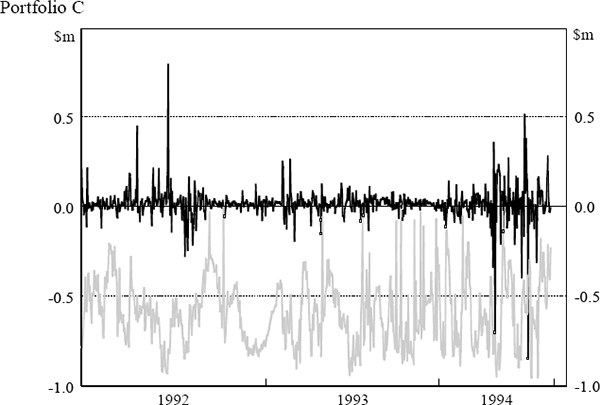
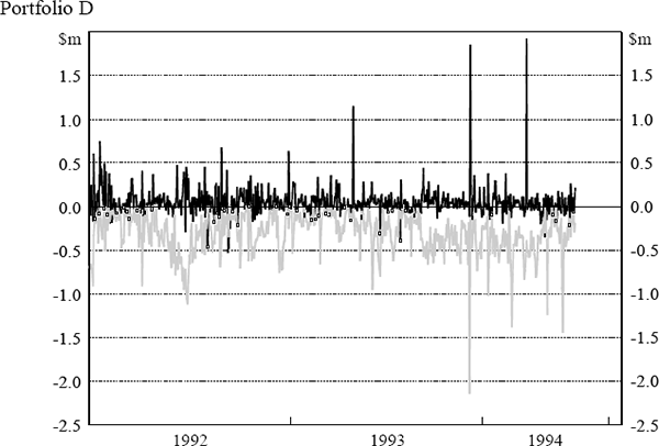
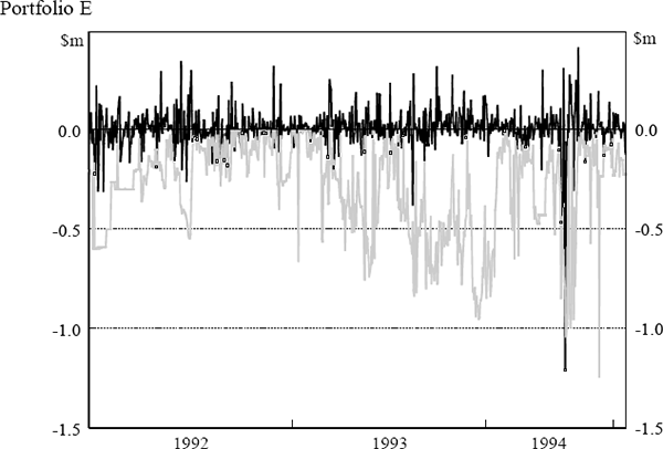
The daily VaR figures were obtained from the daily market risk reports produced by the bank. The reports detail both the bank's total VaR amount and the VaR for individual portfolios (spot foreign exchange (portfolio A), government securities (portfolio B), money market instruments (portfolio C), interest-rate swaps (portfolio D) and interest-rate options (portfolio E)). The testing here assesses VaR model performance at the individual portfolio level. Similarly, profit and loss results were obtained from the bank's internal management report detailing the profit performance of each portfolio. Actual, rather than hypothetical, profit and loss figures have been used. Hence, the profit and loss numbers include some fee income and other income not due to position taking. The daily VaR and profit and loss results for each portfolio are shown in Figure 5. The black lines depict daily profit and loss while the grey lines depict VaR results. Days where the actual loss exceeded the VaR estimate are highlighted.
3.3 The Regulatory Backtest
Backtesting is a fundamental part of the market risk capital standards currently being put in place by supervisors around the world. Under the capital adequacy arrangements proposed by the Basle Committee, each bank must meet a capital requirement expressed as the higher of: (i) an average of the daily VaR measures on each of the preceding sixty trading days, adjusted by a multiplication factor; and (ii) the bank's previous day's VaR number. The multiplication factor is to be set within a range of 3 to 4 depending on the supervisor's assessment of the bank's risk management practices and on the results of a simple backtest (Basle Committee on Banking Supervision 1996a).[4]
The multiplication factor is determined by the number of times losses exceed the day's VaR figure (termed ‘exceptions’) as set out in Table 8 (Basle Committee on Banking Supervision 1996b). The minimum multiplication factor of 3 is in place to compensate for a number of errors that arise in model implementation: simplifying assumptions, analytical approximations, small sample biases and numerical errors will tend to reduce the true risk coverage of the model (Stahl 1997). The increase in the multiplication factor is then designed to scale up the confidence level implied by the observed number of exceptions to the 99 per cent confidence level desired by regulators. In calculating the number of exceptions, banks will be required to calculate VaR numbers using a one-day holding period, and to compare those VaR numbers with realised profit and loss figures for the previous 250 trading days.
| Number of exceptions (in 250 days) |
Multiplication factor | |
|---|---|---|
| Green zone | 4 or less | 3.00 |
| 5 | 3.40 | |
| 6 | 3.50 | |
| Yellow zone | 7 | 3.65 |
| 8 | 3.75 | |
| 9 | 3.85 | |
| Red zone | 10 or more | 4.00 |
A simple approach to exceptions-based backtesting would be to assume that the selected data period provides a perfect indication of the long-run performance of the model. For example, if a VaR model was supposed to produce 99th percentile risk estimates, observed exceptions on any more than 1 per cent of days could indicate problems with the model. This is not realistic since with a finite number of daily observations it is quite probable that the actual number of times that losses exceed VaR estimates will differ from the percentage implied by the model's confidence interval, even when the model is in fact accurate. Hence, the Basle approach is to allocate banks into three zones based on the number of exceptions observed over 250 trading days. A model which truly covers a 99 per cent confidence interval has only a 5 per cent chance of producing more than four exceptions (yellow zone), and only a 0.01 per cent chance of producing more than ten exceptions (red zone).
Table 9 shows the number of regulatory exceptions and the scaling factor to be applied to each portfolio based on the last 250 days' data in the sample.[5] The regulatory backtest places two portfolios (D and E) in the yellow zone. Results in this range are plausible for both accurate and inaccurate models, although it is more likely that the model is inaccurate. Portfolio B is placed in the red zone which will, under the capital-adequacy framework, lead to an automatic presumption that a problem exists within the VaR model.
| Portfolio | Basle exceptions | Scaling factor |
|---|---|---|
| A | 0 | 3.00 |
| B | 10 | 4.00 |
| C | 2 | 3.00 |
| D | 6 | 3.50 |
| E | 8 | 3.75 |
3.4 Exceptions Testing
Kupiec (1995) presents a more sophisticated approach to the analysis of exceptions based on the observation that a comparison between daily profit or loss outcomes and the corresponding VaR measures gives rise to a binomial experiment. If the actual trading loss exceeds the VaR estimate the result is recorded as a failure (or ‘exception’); conversely, if the actual loss is less than the expected loss (or if the actual trading outcome is positive) the result is recorded as a success.
If it can be assumed that a bank's daily VaR measures are independent, the binomial outcomes represent a sequence of independent Bernoulli trials each with a probability of failure equal to 1 minus the model's specified level of confidence; for example, if the level of confidence is 95 per cent the probability of failure on each trial will be 5 per cent.[6] Hence, testing the accuracy of the model is equivalent to a test of the null hypothesis that the probability of failure on each trial equals the model's specified probability. Kupiec uses two tests to examine this hypothesis – the time between failures test and the proportion of failures test.
3.4.1 Time between failures test
The first test is based on the number of trading days between failures and is applied each time a failure is observed. This test is most useful in the case where a risk manager is monitoring the performance of a VaR model on a daily basis and focusing on the new information provided by the model. For example, a bank's risk manager could consider reviewing the model if a number of exceptions occur in succession. The test is less well suited to an analysis of long runs of ex post data on model performance.
To explain the test in more detail we use the following notation:
ν = the observed time (in days) between failures;
p = true probability covered by the VaR model;
p* = the probability specified by the VaR model being tested, (100 – confidence interval)%; and
 = the maximum likelihood estimator of p, given by 1/ν in the
test.
It can be shown that a likelihood ratio (LR) test is the most powerful for testing the null hypothesis that p = p*. The LR statistic is given by:
The LR statistic is distributed as a chi square distribution with 1 degree of freedom.
This test is subject to a number of shortcomings. Firstly, the test has extremely poor power. This means that the test may not reject a VaR model although it continually underestimates risk. The problem is compounded by the fact that the power of the time between failures test is lower, the lower is the probability value under the null hypothesis. That is, for banks with higher stated confidence levels, the likelihood of not rejecting the VaR model, when it is in fact underestimating risk, increases. Moreover, as the VaR model's confidence level increases, the extent by which potential loss is underestimated increases at an accelerating rate. For example, a VaR model purporting to cover a probability of 0.005 but which is in fact generating potential loss estimates consistent with a probability level of 0.025 will underestimate risk by a greater amount than a model with a specified probability level of 0.03 but which yields true coverage consistent with a 0.05 probability.
A second difficulty relates to the values of ν (the number of days between successive failures) associated with the critical value of the LR statistic. The critical value of the distribution, at a 5 per cent level of significance, is 3.841. For a model which specifies a probability level of, say, 0.025 the LR statistic will exceed the critical value (and so the VaR model will be rejected) when ν is less than 12 or greater than 878. For values of ν less than 12, the test concludes that the model is underestimating risk. Conversely, for values of ν greater than 878 the model is likely to be overestimating risk. From a supervisory perspective, the concern is on the former of these alternatives. The problem arises when the specified probability level is 0.05 or larger. In this case, the resulting LR statistic will be less than the critical value for values of ν of two or larger and will be undefined for ν equal to one (when two failures are observed on successive trading days). Hence, for these models there exists no critical value for ν at which the model will be rejected.
Table 10 summarises, for each portfolio, the results of the time between failures test. The second column of the table reports the trading day on which the first failure is observed and column three reveals whether or not the test would reject the model after observing this first failure. Column four lists, for each portfolio, the number of failures that were observed before the VaR model is rejected. Columns five and six report the total number of failures observed over the sample period and the total number of times the null hypothesis was rejected at a 5 per cent level of significance.
| Portfolio |
First failure |
Test result |
Failures before first rejection |
Failures |
Rejections |
|---|---|---|---|---|---|
| A | 4 | reject | 1 | 5 | 3 |
| B | 5 | reject | 1 | 27 | 17 |
| C | 203 | do not reject | – | 3 | 0 |
| D | 28 | do not reject | 2 | 31 | 17 |
| E | 88 | do not reject | 4 | 36 | 24 |
The results in Table 10 imply that the model performs well for portfolios A and C while portfolios B, D and E are identified as portfolios where the model does not seem to be adequately capturing the potential for losses to be observed. There are a number of occasions on which these three portfolios experience a run of rejections on successive trading days or trading days two or three days apart. This result suggests that the VaR model may not be able to cope with large movements in market prices; it could be that the price volatilities within the VaR are not updated with sufficient frequency to capture the time-varying nature of the profit and loss variability (that is, autoregressive conditional heteroscedasticity). It is noteworthy that if this LR test was applied by a risk manager to performance data on a daily basis this problem with the model would be detected quite early on in the sample period.
3.4.2 Proportion of failures test
The second test is based on the proportion of failures observed over the entire sample period. A test of the null hypothesis that the VaR model's stated probability level is equal to the realised probability level covered by the VaR model (p = p*) is again best achieved using a LR test. The LR test statistic is given by:
where n denotes the total number of outcomes in the sample period, x
denotes a Bernoulli random variable representing the total number of observed
failures and  is the maximum likelihood estimator, given
by x/n (x ≥ 1).
While this test is better suited to an analysis of ex post data than is the time between failures test, it still has some problems. As was the case with the preceding test, the proportion of failures test has poor power characteristics which become worse as the confidence interval being tested increases. Further, although the power of the test improves as the sample period increases, a substantial sample size is required for the test to have significant power. Nonetheless, with the exception of the case of a single failure for which the test is equivalent to the time between failures test, the proportion of failures test has more power than the preceding test owing to its making use of more information. Moreover, the LR statistic is defined for all combinations of x and n (except x = n = 1) and so can be applied for all stated probabilities.
Table 11 summarises the results of the proportion of failures test when applied to each of the portfolios. As with the time between failures test, it can be concluded that those portfolios whose models do not give rise to any failures over the period are not rejected. For all portfolios the results of this test are consistent with the time between failures test.
| Portfolio | x | n | Proportion of failures (%) | Chi square | Significance |
|---|---|---|---|---|---|
| A | 5 | 653 | 0.8 | 0.8 | 0.372 |
| B | 27 | 673 | 4.0 | 66.0 | 0.000 |
| C | 3 | 669 | 0.4 | 0.0 | 0.847 |
| D | 31 | 631 | 4.9 | 87.2 | 0.000 |
| E | 36 | 692 | 5.2 | 105.1 | 0.000 |
3.5 Estimates of Variance
A VaR figure can be regarded simply as a rescaled variance. This is most transparent in the variance-covariance calculation of VaR. Hence, it is possible to undo a VaR calculation to obtain the profit and loss volatility underlying the VaR calculation and to compare this against the observed variance of profits and losses. The test below compares the volatility derived from the average VaR over time with the variance of the actual profit and loss distribution over the same period. Assuming that profits and losses are normally distributed (the validity of this assumption is tested in the next section), an F test can be used to test whether the two variance estimates are significantly different. Under the null hypothesis that the variances are equal the ratio of the estimates follows an F distribution:
where  denotes the average VaR over time, k denotes the number of standard deviations
required for the specified confidence interval (for example, a 97.5 per cent
confidence interval is equivalent to 1.96 standard deviations) and n
denotes the number of daily observations.
Table 12 which follows shows the observed standard deviation of profit and loss,
 and the results of the F test for each portfolio. For all portfolios, except portfolio
D, the VaR variance is not significantly less than the profit and loss variance
suggesting that overall the VaR adequately captures true volatility.
| Portfolio |  |
P&L Std Dev ($ 000) | F | Significance |
|---|---|---|---|---|
| A | 417.3 | 152.9 | 0.134 | 1.000 |
| B | 123.9 | 110.0 | 0.788 | 0.999 |
| C | 229.6 | 92.2 | 0.161 | 1.000 |
| D | 118.1 | 172.4 | 2.129 | 0.000 |
| E | 113.1 | 101.2 | 0.800 | 0.998 |
3.6 Tests of Normality
Where it is the case that a bank uses a VaR methodology that assumes that financial returns are normally distributed (such as the variance-covariance method), testing whether the observed profits and losses follow a normal distribution can serve as useful backtesting.
There is a wide variety of tests that may be used to test for normality. Two of the simplest tests focus on the skewness and kurtosis of the observed distribution.
Skewness measures the imbalance in a distribution, that is, whether observations occur more frequently above or below the mean. The skewness of each profit and loss series and the result of tests to determine whether the skewness is significantly non-zero are presented in Table 13. Tests for the significance of the skewness statistic are set out in Kendall and Stuart (1963).
| Portfolio | Skew | Significance | Kurtosis | Significance | KS | Significance | Kuiper | Significance |
|---|---|---|---|---|---|---|---|---|
| A | −0.462 | 0.000 | 3.292 | 0.000 | 1.307 | 0.066 | 2.627 | 0.000 |
| B | 2.347 | 0.000 | 41.477 | 0.000 | 4.087 | 0.000 | 8.212 | 0.000 |
| C | −1.029 | 0.000 | 30.396 | 0.000 | 4.710 | 0.000 | 9.243 | 0.000 |
| D | 4.472 | 0.000 | 42.118 | 0.000 | 3.939 | 0.000 | 6.868 | 0.000 |
| E | −2.598 | 0.000 | 32.455 | 0.000 | 3.042 | 0.000 | 5.976 | 0.000 |
| Total bank | 0.983 | 0.000 | 7.939 | 0.000 | 1.705 | 0.006 | 3.142 | 0.000 |
In the opening section of this paper it was shown that large exchange rate movements are observed more often than is consistent with the data being normally distributed; that is, the empirical distributions for exchange rates have fatter tails than the normal distribution. In fact, it has been observed that a large number of financial series exhibit fat tails (see, for example, Bollerslev et al. (1994)). It is possible to quantify the divergence between the tails of the observed and normal distributions by measuring the kurtosis of the observed distribution as:
If ν4 = 0 the tails on the distribution follow a normal distribution, if ν4 is negative the distribution has thinner tails than a normal distribution, while if ν4 is positive the distribution has fatter tails (known as leptokurtosis). Again, tests for the significance of the kurtosis statistic are given in Kendall and Stuart (1963).
Tests based on skewness and kurtosis each focus on one particular aspect of the observed distribution. It is also possible to devise tests that take into account the entire distribution by comparing the cumulative distribution functions of the observed data and the normal distribution. As an example, Figure 6 shows the observed cumulative distribution function for the profits and losses on portfolio A compared with the standard normal cumulative distribution function. There are a number of ways to quantify the difference between the two functions. One widely used test is the Kolmogorov-Smirnov test which takes as its test statistic the maximum value of the absolute difference between the two functions (the distance between points A and B in Figure 6).
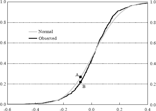
One weakness with this test is that it places greater weight on observations around the median. An alternative test which gives equal weight to all percentiles across the distribution is the Kuiper test (Crnkovic and Drachman 1996). This test is based on the statistic:
where S(·) is the observed cumulative distribution function, N(·) is the Normal cumulative distribution function and x denotes observations of profit and loss results.[7] That is, instead of looking at the largest distance between the functions, the Kuiper statistic takes into account the sum of the maximum distance of S(x) above N(x) and below N(x). Press et al. (1992) describe the procedures for testing the significance of the Kolmogorov-Smirnov and Kuiper statistics.
The skewness and kurtosis statistics, along with tests of their significance, and the results of Kolmogorov-Smirnov (KS) and Kuiper tests are presented in Table 13. The results of the four tests are in agreement; the tests yield a consistent conclusion for all five portfolios. All portfolios are found to be strongly non-normal. Since a variance-covariance VaR model is used by the bank, the finding of non-normality implies that the VaR measure will not correctly estimate the true risk exposure. In particular, since the profit and loss distributions are quite fat-tailed, the VaR model would be expected to significantly underestimate risk.
Given that the bank's profit and loss data does include fee income and other income derived from the bid/offer spread that a market maker is able to obtain, some negative skewness in the profit and loss distribution would be expected. In fact the test results are quite mixed, with two of the five portfolios exhibiting positive skewness. To the extent that there is positive skewness in the profit and loss distribution, the variance-covariance VaR calculation will overestimate true risk, offsetting any underestimation resulting from the failure to capture the leptokurtosis (fat tails) of the distribution.
Given that individual portfolios may be quite non-normal, this could result in VaR models that do assume normality significantly underestimating risk. It is at the aggregate level (that is, the sum of individual portfolio's profit and loss), however, that regulatory tests will apply in the first instance. It is expected that non-normality should be less evident at the aggregate level than for individual portfolios. This is based on the central limit theorem which states that taking the sum of increasing numbers of individual statistical processes will result in the distribution of the sum tending towards normality regardless of the distribution of the individual components. In fact, as shown in Table 13, this effect does not seem to be very strong. The total profit and loss for the bank remains strongly non-normal.
3.7 Risk Tracking
There are two dimensions to evaluating the performance of any risk measure – the level of coverage provided and the efficiency of the measure. The tests in the previous sections have focused on coverage – what level of losses would a VaR-based capital charge insure against. A good risk measure needs to be more than just appropriately conservative, it should also be strongly correlated with the portfolio's true risk exposure. A conservative but inefficient risk measure would tend to overestimate risk in periods of low risk.
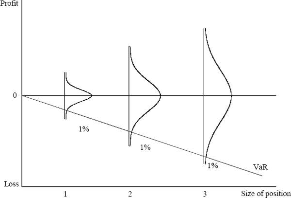
The very simplest test that can be performed is to assess the relationship between the VaR estimates and the absolute value of each day's profit or loss. In a very simple sense, large VaR figures should be accompanied by large profits or losses while small VaR estimates should be associated with small profit and loss results. Consider a portfolio containing positions in a single asset: as the exposure to that asset grows the variance of the profit and loss distribution will increase and the VaR should increase to reflect the greater exposure (Figure 7). As the exposure increases, larger profit and loss observations become more likely. To the extent that the VaR is tracking the increased variance of the underlying profit and loss distribution, there should be some correlation between the size of profits and losses and the VaR. This effect may not be strong, however, as the bulk of the profit and loss observations will be drawn from the centre of the distribution.
In the broadest terms, both VaR and profit and loss are a function of two processes – changes in market prices and the composition of the bank's portfolio. The bank considered here uses a relatively long run of data to calculate historical price volatilities and updates the price volatility history quarterly. The bank does not use a time weighting scheme such as exponential weighting but rather assumes that the covariance matrix is fixed independent of time. As a result, the bulk of the time variation in the VaR figures comes from changes in the composition of the bank's portfolios.
If the bank's portfolios were constant (and assuming that the statistical process driving market prices are unchanging through time), then the profit and loss distributions would be constant through time. A perfectly efficient VaR, in such a case, would also be constant. Hence, profit and loss magnitudes and VaR estimates would be quite uncorrelated despite the fact that the VaR is perfectly efficient. However, banks' portfolios are not constant; as can be seen from Figure 5, the bank considered here is an active trader whose portfolio composition and profit and loss distribution change markedly from day to day.
Given that the assumption of normality of both the absolute value of profit and loss
and VaR is problematical, it is useful to consider tests which do not require
any assumption about the distribution of the two series. One such test is based
on the rank correlation coefficient. Let X denote the series of profit and
loss magnitudes and Y the VaR series. Ranks 1, 2, …, n are then assigned to the X's and Y's. Let Ui
= rank of Xi and Vi = rank of Yi then the
rank correlation coefficient, R, is defined as the correlation between U and
V. For sufficiently large samples  . Tests of the significance of the relation
between the two series can be based on this.
The rank correlations for each portfolio are presented in Table 14. Overall, the tests indicate that the VaR numbers are not strongly correlated with the magnitudes of the profit and loss outcomes. While four of the five rank correlations are significantly positive, the magnitude of the estimated correlations are small.
| Portfolio | Rank correlation | Significance |
|---|---|---|
| A | 0.142 | 0.000 |
| B | 0.240 | 0.000 |
| C | 0.129 | 0.001 |
| D | 0.017 | 0.672 |
| E | 0.182 | 0.000 |
Footnotes
The market risk capital adequacy arrangements to apply to Australian banks (Prudential Statement No. C3) were released by the Reserve Bank in January 1997 and are broadly consistent with the Basle Committee's international standards. [4]
For internal risk management purposes the bank does not use a 99 per cent confidence interval; the Basle exceptions were calculated using VaR figures that had been rescaled to 99 per cent confidence equivalent amounts. All subsequent testing is based on the bank's own internal confidence level. [5]
In fact this is not a good assumption. The Ljung-Box Q-test for serial correlation found significant autocorrelation in the VaR series for all five portfolios. [6]
An unbiased estimator of the cumulative distribution function of the probability distribution from which the profit and loss figures are drawn, S(x), is given by the fraction (out of the total number of observations) of data points that are less than x. [7]


