RDP 9708: Measuring Traded Market Risk: Value-at-risk and Backtesting Techniques 2. Value-at-risk
November 1997
- Download the Paper 400KB
Internationally the use of VaR techniques has spread rapidly. This section defines the VaR measure and discusses its use within the Australian banking industry. We then discuss the three methods most commonly used to calculate a VaR estimate – the variance-covariance approach, the historical-simulation approach and the Monte-Carlo simulation approach.
In addition to its inclusion in the Basle Committee on Banking Supervision's guidelines for market risk capital adequacy,[1] a number of other official bodies and industry groups have recognised VaR as an important market-risk measurement tool. For example, the ‘Fisher Report’ (Euro-currency Standing Committee 1994) issued by the Bank for International Settlements in September 1994 made recommendations concerning the disclosure of market risk by financial intermediaries and advocated the disclosure of VaR numbers in financial institutions' published annual reports. Moreover, private-sector organisations such as the Group of Thirty (1993) (an international group of bankers and other derivatives market participants) have recommended the use of VaR methodologies when setting out best-practice risk-management standards for financial institutions.
VaR is one of the most widely used market risk-measurement techniques by banks, other financial institutions and, increasingly, corporates. Of the banks visited by the Reserve Bank's Market-Risk On-Site review team as at end October 1997, more than half had some form of VaR calculation in place.
The application of VaR techniques is usually limited to assessing the risks being run in banks' treasury or trading operations (such as securities, foreign exchange and equities trading). It is rarely only applied to the measurement of the exposure to the interest-rate and foreign-exchange risks that arise from more traditional non-traded banking business (for example, lending and deposit taking). Use of VaR by Australian banks ranges from a fully integrated approach (where VaR is central to the measurement and internal reporting of traded market risk and VaR-based limits are set for each individual trader) to an approach where reliance is placed on other techniques and VaR is calculated only for the information of senior management or annual reporting requirements. At this stage, it is most common to see VaR used to aggregate exposures arising from different areas of a bank's trading activities while individual traders manage risk based on simpler, market-specific risk measures.
2.1 Defining Value-at-risk
Value-at-risk aims to measure the potential loss on a portfolio that would result if relatively large adverse price movements were to occur.[2] Hence, at its simplest, VaR requires the revaluation of a portfolio using a set of given price shifts. Statistical techniques are used to select the size of those price shifts.
To quantify potential loss (and the severity of the adverse price move to be used) two underlying parameters must be specified – the holding period under consideration and the desired statistical confidence interval. The holding period refers to the time frame over which changes in portfolio value are measured – is the bank concerned with the potential to lose money over, say, one day, one week or one year. For example, a VaR measure based on a one-day holding period reflects the impact of daily price movements on a portfolio. It is assumed that the portfolio is held constant over the holding period. The Basle Committee's standards require that banks use a ten-day holding period – thus requiring banks to apply ten-day price movements to their portfolios. The confidence level defines the proportion of trading losses that are covered by the VaR amount. For example, if a bank calculates its VaR assuming a one-day holding period and a 99 per cent confidence interval then it is to be expected that, on average, trading losses will exceed the VaR figure on one occasion in one hundred trading days.
Thus, VaR is the dollar amount that portfolio losses are not expected to exceed, with a specified degree of statistical confidence, over a pre-specified period of time.
2.2 An Example Portfolio
A simple portfolio of two spot foreign-exchange positions can be used to illustrate and compare three of the most common approaches to the calculation of VaR. In the following examples, a one-day holding period is assumed and VaR is defined in terms of both 95th and 99th percentile confidence levels.
The example portfolio consists of a spot long position in Japanese Yen and a spot short position in US dollars (Table 1). Thus the value of the portfolio will be affected by movements in the JPY/AUD and USD/AUD exchange rates.
| Position 1 | 100,000 | JPY long |
|---|---|---|
| Position 2 | −10,000 | USD short |
Estimation of a VaR figure is based on the historical behaviour of those market prices that affect the value of the portfolio. In line with the Basle Committee's requirements we use 250 days of historical data, from 9 June 1995 to 5 June 1996, to perform the VaR calculations below.
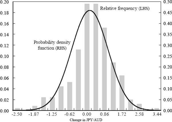
Figures 1 and 2 are histograms of the daily returns for the JPY/AUD and USD/AUD exchange rates. The smooth line in each chart represents a normal distribution with the same mean and standard deviation as the data. In both the upper and lower tails of each series, the actual frequency of returns is greater than that which would be expected if returns were normally distributed (that is, the observed distributions of daily returns have ‘fatter tails’ than implied by the normal distribution). Thus both series of daily returns appear more likely to be samples drawn from some distribution other than a normal distribution (such as a t-distribution). The implications of this result for the calculation of a VaR number will be considered later in this paper.

The starting point of all three VaR approaches is to revalue the portfolio at current market prices. Table 2 shows the revalued portfolio given the foreign exchange rates on 5 June 1996.
| Spot FX rate | Position value | AUD equivalent | |
|---|---|---|---|
| Position 1 | JPY/AUD 86.46 | 100,000 JPY | 1,156.60 (100,000/86.46) |
| Position 2 | USD/AUD 0.7943 | −10,000 USD | −12,589.70 (−10,000/0.7943) |
2.3 The Variance-covariance Approach
In terms of the computation required, the variance-covariance method is the simplest of the VaR approaches. For this reason, it is often used by globally active banks which need to aggregate data from a large number of trading sites. Variance-covariance VaR was the first of the VaR approaches to be offered in off-the-shelf computer packages and hence, is also widely used by banks with comparatively low levels of trading activity.
The variance-covariance approach is based on the assumption that financial-asset returns and hence, portfolio profits and losses are normally distributed. The consequence of these two assumptions is that VaR can be expressed as a function of:
- the variance-covariance matrix for market-price returns; and
- the sensitivity of the portfolio to price shifts.
The first stage of the variance-covariance approach requires the calculation of a variance-covariance matrix using the 250 days of historical data for the two series of daily exchange rate returns. The variance-covariance matrix for this example is expressed as:
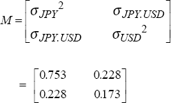
where σJPY2 is the variance of the series of daily returns for JPY/AUD, σUSD2 is the variance of the series of daily returns for USD/AUD and σJPY.USD is the covariance between the two series.
The second step in this approach is to calculate the market price sensitivities or deltas of the portfolio; that is, the amounts by which the portfolio's value will change if each of the underlying market prices change by some pre-specified amount. To do this, movements in each of the market prices which affect the value of the portfolio are examined separately. Table 3 shows the change in the portfolio given a 1 per cent move in each of the spot FX rates.
| Current | Revalued (assuming a 1% increase in AUD) | ||
|---|---|---|---|
| FX rates | |||
| JPY/AUD | 86.46 | 87.32 | (1.01 × 86.46) |
| USD/AUD | 0.7943 | 0.8022 | (1.01 × 0.7943) |
| Portfolio value (AUD) | |||
| Position 1 | 1,156.61 | 1,145.15 | (100,000 / 87.32) |
| Position 2 | −12,589.70 | −12,465.05 | (−10,000 / 0.8022) |
| Change in portfolio value or delta (AUD) | |||
| Position 1 | −11.45 | ||
| Position 2 | 124.65 | ||
The third step in this approach is to calculate the standard deviation or volatility of total changes in portfolio value. Since total portfolio changes are assumed to be normally distributed, the volatility of portfolio changes can be expressed as a function of the deltas, the standard deviations of the two market-factor returns and the covariance between them. Let δ be the vector of market-price sensitivities or deltas. If the standard deviation of portfolio changes is ν and the variance-covariance matrix of the market prices is M then ν is expressed as:

In this example ν is given by:
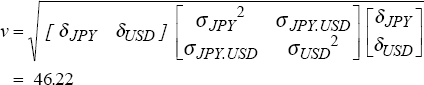
The standard deviation of changes in the portfolio's total value is 46 AUD.
To establish the VaR number of the portfolio for a given level of confidence the standard deviation must be multiplied by the relevant scaling factor, which is derived from the standard normal distribution. For example, if a 99 per cent level of confidence is desired the appropriate scaling factor is 2.33 since the probability of occurrence of a number less than −2.33 is 1 per cent. Scaling the standard deviation of the portfolio by this amount yields a VaR number which should only be exceeded 1 per cent of the time. Note that the choice of a 99 per cent confidence level and associated scaling factor of 2.33 assumes a one-tailed test in line with the Basle market risk requirements (that is, only large losses are considered, not large profits).
Table 4 shows the VaR amounts, given 95 and 99 per cent levels of confidence, for the example portfolio. Clearly the higher the level of confidence, the larger the VaR number will be: given the various assumptions there is a 5 per cent probability that the loss on the portfolio will exceed 76 AUD and only a 1 per cent probability that the loss on the portfolio will be larger than 108 AUD.
| Confidence level | Scaling factor | Value-at-risk number |
|---|---|---|
| 95 per cent | 1.645 | 76.02 AUD (46.21×1.645) |
| 99 per cent | 2.330 | 107.67 AUD (46.21×2.33) |
2.4 The Historical-simulation Approach
The historical-simulation method is more computationally intensive than the variance-covariance approach and its use emerged within the Australian banking industry a little later. While only three banks have been using historical simulation for some time, the development of historical databases of market prices, together with more powerful (and less expensive) computer technology, has led several other banks to move towards the use of this approach.
The historical-simulation approach also uses historical data on daily returns to establish a VaR number, however, it makes no assumptions about the statistical distribution of these returns. The first step in this approach is to apply each of the past 250 pairs of daily exchange rate movements to the portfolio to determine the series of daily changes in portfolio value that would have been realised had the current portfolio been held unchanged throughout those 250 trading days.
To determine the revalued portfolio value two approaches can be used. The simpler approach requires the previously calculated delta amount for each position to be multiplied by each of the past changes in the relevant exchange rate. Recall that delta measures how much the position value will change if the exchange rate changes by 1 per cent. If the past actual change in the exchange rate is, say, 0.16 per cent then the portfolio value will change by 0.16 × delta. The second, more arduous approach is to revalue each position in the portfolio at each of the past exchange rates. For linear positions (that is, positions the values of which change linearly with changes in the underlying market prices) the two approaches will yield the same result. However, for non-linear positions, such as positions in complex options, the first approach may substantially under or overestimate the change in the value of the position and thus may not generate an accurate measure of market risk exposure.
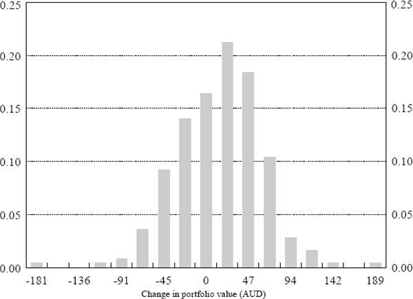
The second step is to sort the 250 changes in portfolio value in ascending order to arrive at an observed distribution of changes in portfolio value. The histogram of these changes is shown in Figure 3. The VaR number will be equal to that percentile associated with the specified level of confidence. For a 95 per cent level of confidence, the VaR number is 68.17 AUD and equals the 5th percentile of the distribution of changes in portfolio value. The kth percentile means that the lowest k per cent of the sample of changes in portfolio value will exceed the VaR measure. Since there are 250 observations, essentially this means that 12.5 losses (or 5 per cent of the sample) will be larger than the VaR measure (the VaR measure is essentially the 13.5 lowest observation). Similarly, for a 99 per cent level of confidence the VaR number is 102.11 and equals the first percentile. These results are summarised in Table 5.
| Confidence level | Value-at-risk number |
|---|---|
| 95 per cent | 68.17 AUD |
| 99 per cent | 102.11 AUD |
2.5 Monte-Carlo Simulation
This method is not widely used by Australian banks. Monte-Carlo techniques are extremely computer intensive and the additional information that these techniques provide is of most use for the analysis of complex options portfolios. To date, use of Monte-Carlo simulation has been limited principally to the most sophisticated banks and securities houses operating in the US. The Monte-Carlo method is based on the generation, or simulation, of a large number of possible future price changes that could affect the value of the portfolio. The resulting changes in portfolio value are then analysed to arrive at a single VaR number.
Briefly, the method requires the following steps.
- A statistical model of the market factor returns must be selected and the parameters of that model need to be estimated. For the purposes of our example, it is assumed that the two exchange-rate returns are drawn from a bivariate t-distribution with 5 degrees of freedom and a correlation of 0.63.[3] A t-distribution was chosen as it is able to capture the fat-tails characteristic observed in the data.
- A large number of random draws from the estimated statistical model are simulated. This is done using a sampling methodology called Monte-Carlo simulation in which a mathematical formula is used to generate series of ‘pseudo-random’ numbers to simulate the market factors. In this example, the two exchange rates are simulated 50,000 times.
- The portfolio is revalued for each pair of simulated exchange rates and the changes in portfolio value between the current value and these revalued amounts are then determined. Figure 4 shows the histogram of these changes.
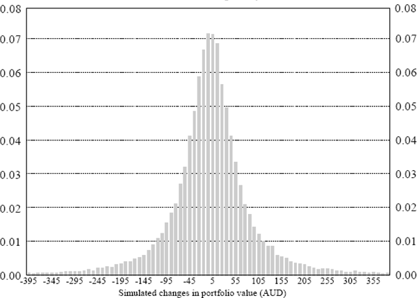
In the same way as in the historical simulation approach, these changes in portfolio value are sorted in ascending order and the VaR number at a k per cent level of confidence is determined as the (100-k) percentile of these sorted changes. The resulting VaR measures are shown in Table 6.
| Confidence level | Value-at-risk number |
|---|---|
| 95 per cent | 157.96 AUD |
| 99 per cent | 356.10 AUD |
The Monte-Carlo process permits analysis of the impact of events that were not in fact observed over the historical period but that are just as likely to occur as events that were observed. It is this capacity to evaluate likely events that have not occurred that is one of the main attractions of this approach.
2.6 A Comparison of the Three Methods
The VaR numbers derived from the three approaches produce a wide range of results (Table 7). In this example, the historical simulation method which takes into account the actual shape of the observed distribution of profits and losses (shown in Figure 3) yields the lowest risk estimates. The variance-covariance method's assumption of symmetry around a zero mean gives equal weight to both profits and losses, resulting in VaR estimates which are slightly higher than those of the historical simulation approach. The simulation of a bivariate t-distribution results in VaR estimates which are much larger than the estimates given by the other two methods. A t-distribution with the same mean and variance as a normal distribution will have a greater proportion of its probability mass in the tails of the distribution (in fact, in this case, the t-distribution also has longer tails than the empirical distribution). The prime focus of a VaR model is the probability of tail events, hence, the long tails of the t-distribution have a disproportionate effect on the VaR estimate. It can be seen that this effect becomes more marked the higher the confidence level. It should be noted that this ranking of results from the three methods is dependent on the data and also the statistical distribution used within the Monte-Carlo simulation technique. Other price series exhibiting different mean, skew and tail characteristics may result in the relative sizes of the three methods' VaR estimates being quite different.
| 95 per cent | 99 per cent | |
|---|---|---|
| Variance-covariance | 76.02 AUD | 107.67 AUD |
| Historical-simulation | 68.17 AUD | 102.11 AUD |
| Monte-Carlo simulation | 157.96 AUD | 356.10 AUD |
2.7 Advantages and Shortcomings of VaR
While VaR is used by numerous financial institutions it is not without its shortcomings. First, the VaR estimate is based solely on historical data. To the extent that the past may not be a good predictor of the future, the VaR measure may under or overestimate risk. There is a continuing debate within the financial community as to whether the correlations between different financial prices are sufficiently stable to be relied upon when quantifying risk. There is also debate as to how best to model the behaviour of volatility in market prices. Nevertheless, if an institution wishes to avoid relying on subjective judgments regarding likely future financial market volatility, reliance on history is necessary.
Second, a VaR figure provides no indication of the magnitude of losses that may result if prices move by an amount which is more adverse than that amount dictated by the chosen confidence level. For example, the dollar VaR provides no insight into what would happen to a bank if a 1 in 10,000 chance event occurred. To address the risks associated with such large price shifts, banks are developing, and bank supervisors are requiring, more subjective approaches such as stress testing to be adopted in addition to the statistically based VaR approach. Stress testing involves the specification of stress scenarios (for example, the suspension of the European exchange rate mechanism) and analysis of how banks' portfolios would behave under such scenarios.
Third, the comparative simplicity of a VaR calculation where exposures in a wide array of instruments and markets can be condensed into a single figure is both a strength and a weakness. This simplicity has been the key to the popularity of VaR, particularly as a means of providing summary information to a bank's senior management. The difficulty with this though, is that such a highly aggregate figure may mask imbalances in risk exposure across markets or individual traders.
One of the chief advantages of the VaR approach is that it assesses exposure to different markets (interest rates, foreign exchange, etc) in terms of a common base – losses relative to a standard unit of likelihood. Hence, risks across different instruments, traders and markets can be readily compared and aggregated. In addition, a dollar-value VaR can be directly compared to actual trading profit and loss results – both as a means of testing the adequacy of the VaR model and to assess risk-adjusted performance. Risk-adjusted returns can be quantified simply by looking at the ratio of realised profits/losses to VaR exposure. Such calculations provide a basis for a bank to develop sophisticated capital-allocation models and to renumerate individual traders not just for the volume of trading done, but to reflect the riskiness of each trader's activities.
Footnotes
Basle Committee on Banking Supervision (1996a, 1996b). [1]
Value-at-risk may also be termed earnings-at-risk or a potential loss amount. [2]
Maximum likelihood estimation of the degrees of freedom for a univariate t-distribution for each of the exchange rate returns series yielded an estimate of 5 degrees of freedom for both the USD/AUD and the JPY/AUD rates. [3]