RDP 9210: Contingent Claim Analysis of Risk-Based Capital Standards for Banks 3. Two Risk-Based Capital Rules

Within the context of our model, risk-based capital requirements specify a relationship between the capital ratio c ≡ (V₀−D₀)/V₀ and asset risk σ. The exact form of the relationship depends on the regulatory goal being pursued.

3.1 A Liability-Value Rule

One possible regulatory goal that risk-based capital standards could be designed to achieve is to maintain the contingent liability of the deposit guarantor at some fixed level relative to deposits, irrespective of banks' operating decisions. (This goal might be especially attractive in countries such as the United States that meet the cost of the guarantee through a deposit-based assessment on the banking system.) Dividing both sides of equation (2) by D₀ yields the liability per dollar of bank deposits, which we denote LV:

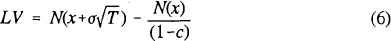
where x is as defined in (3), noting that D₀/V₀ = 1−c. Equation (6) shows that the guarantor's liability per dollar of deposits depends only on asset risk σ, the time to the monitoring date T, and the capital ratio c; it is independent of bank size and interest rates.

Level curves LV(σ,c)=LV₀ give combinations of σ and c that yield the same liability of LV₀ per dollar of deposits. Examples of these curves are shown in Figure 1, with T=1. It is easily shown that LV(σ,c) is increasing in σ and decreasing in c; in words, the guarantor's liability is greater for higher levels of asset risk and for lower values of the capital ratio. Thus a risk-based capital rule designed to limit the liability imposed by individual banks would allow (σ,c) combinations on or to the left of one of the level curves.

A general expression for the slope of the level curves can be obtained by taking the total differential of LV(σ,c), setting it equal to zero, and rearranging to obtain dc/dσ:

where n(•) is the standard normal density function. For a bank that is on the boundary of allowable combinations of σ and c, expression (8) specifies the increase in capital that would be required for a small increase in asset risk. This positive relationship between risk and capital provides the basis for an LV risk-based capital standard. Of course, (8) only gives the slope of the risk-based capital schedule that holds the liability constant. Policy makers also would have to determine an acceptable level of LV₀ to construct a complete regulatory standard. For a given value of the liability LV₀ and a given monitoring period T, (8) defines the capital ratio as an implicit increasing function of asset risk.

3.2 A Failure-Probability Rule

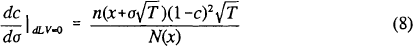
Level curves FP(σ,c)=FP₀ of the failure probability function give combinations of σ and c that yield a constant probability of failure equal to FP₀. Three examples are plotted in Figure 2, with T again set equal to one. Like the per-dollar contingent liability, FP(σ,c) is decreasing in c, and generally is increasing in σ.^[4] An FP risk-based capital rule designed to limit the probability of failure would allow (σ,c) combinations on or to the left of one of the constant failure probability curves.

To derive the slope of a failure probability locus we take the total differential of 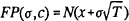and set it equal to zero:

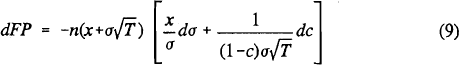
For a bank on the boundary of allowable combinations of σ and c, expression (10) defines c implicitly as a function of σ, and hence specifies the increase in capital required for a small increase in asset risk. As with an LV rule, regulators would need to determine an acceptable value of FP₀ to actually implement a policy based on this relationship.

3.3 Comparing the Two Rules

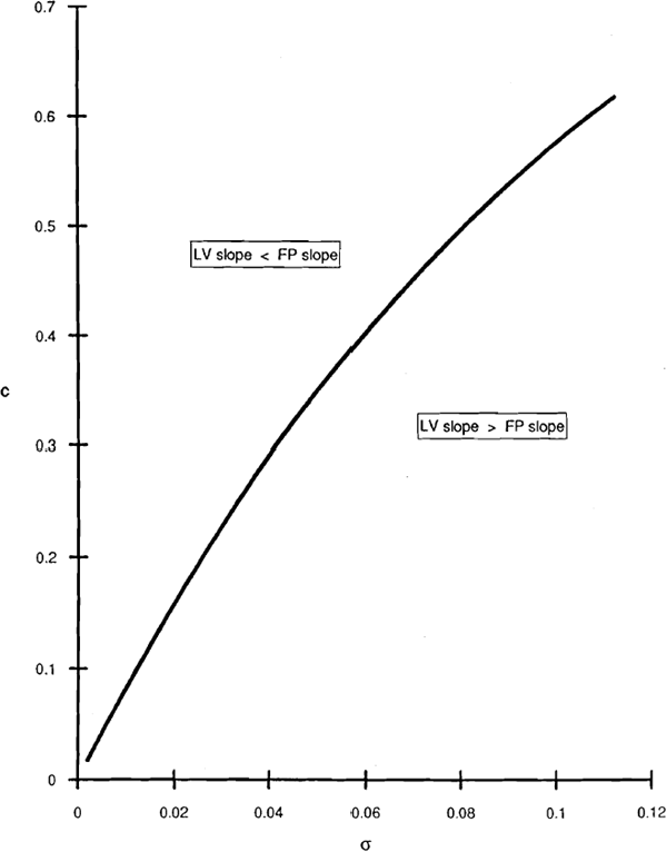
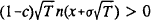
The two risk-based capital standards described above differ in the size of the increase in capital required for any given increase in asset risk. Any combination of σ and c that a bank might select lies on both an LV locus and an FP locus. Comparison of (8) and (10) reveals that a sufficient condition for dc/dσ to be greater along the liability-value locus than along the failure-probability locus is n(x)/N(x)+x>0.^[5]

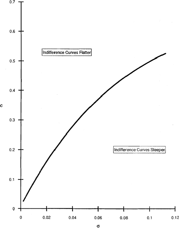
Figure 3 shows combinations of c and σ that make the slopes of the LV and FP loci equal, along the locus labelled n(x)/N(x)+x=0. Above this locus LV curves are flatter than FP; the opposite is true below and to the right of the locus. Casual observation suggests that banks generally have capital and asset risk combinations that put them in the lower part of the figure. Thus the LV curve is likely to be steeper than the FP curve, implying that an LV rule would dictate larger capital responses to changes in operating risk than an FP rule. The difference arises because the FP rule weights all insolvency outcomes equally, while the LV rule gives greater weight to outcomes entailing larger losses for the deposit guarantor.

To compare bank behaviour under the two rules we assume the bank chooses a combination of capital and risk to maximise the value of equity net of contributed capital (V₀−D₀) but inclusive of the implicit put option (L) generated by the guaranteed deposits, subject to the constraint that the capital requirement be met. We assume that changes in the capital ratio are achieved through substitution of capital for deposits, leaving the value of assets unchanged,^[6] and that assets are purchased or originated in competitive markets so that their value is unaffected by the riskiness of the bank. The total value of equity, which we denote E, is given by:

Since contributed capital is V₀−D₀ and the bank maximises E net of contributed capital, the bank's effective objective is to maximise the value of the implicit put option.

If the bank changes its combination of capital and risk, the value of the bank's equity changes according to:

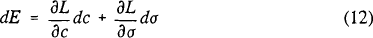
Differentiating the expression for L given in equation (2), and using the definition of c, dE can be rewritten:

Setting dE equal to zero characterises the bank's indifference curves in the (σ,c) plane.^[7] Since and , the net value of bank equity is decreasing in the capital ratio and increasing in asset risk. Thus indifference curves which are downward and to the right in the (σ,c) plane represent higher values of equity.

If the bank's indifference curves are flatter than the boundary implied by the capital standard, the bank will be pushed toward low-risk, low-capital portfolios.^[8] Conversely, if the indifference curves are steeper than that boundary, the bank will be pushed toward high-risk, high-capital portfolios. Setting dE equal to zero and rearranging yields the slope of the bank's indifference curves:

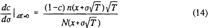
Comparing (8) and (14), the indifference curves are flatter than the LV rule boundary if 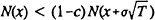; we know this inequality always holds, since . Comparing (10) and (14), the bank's indifference curves are flatter than the FP rule boundary if 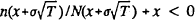. Figure 4 shows the locus of points for which the slopes are just equal. The bank's indifference curves are flatter than the FP locus at points above and to the left, which as noted above are unlikely choices for actual banks. Indeed, these low-risk, high-capital combinations are optimal only if the FP rule requires failure probabilities on the order of 10^-18 or less. In general the relationship between the slopes is likely to be that the LV curves are steeper than the bank's indifference curves, while the FP curves are flatter:

Thus if an LV rule is in place banks will be pushed toward lower-risk, lower-capital portfolios, while an FP rule will push banks toward higher-risk, higher-capital portfolios.

Limiting the probability of bank failure and limiting the liability of the deposit guarantor both are plausible regulatory objectives. Although the two goals are closely related, the contingent claim model suggests that bank behaviour under a policy designed to meet one of these goals may differ markedly from behaviour under a policy designed to meet the other. Moreover, the model suggests that the two regulatory goals may conflict; holding the value of the deposit guarantee liability constant may result in unacceptably high probabilities of failure and vice-versa.

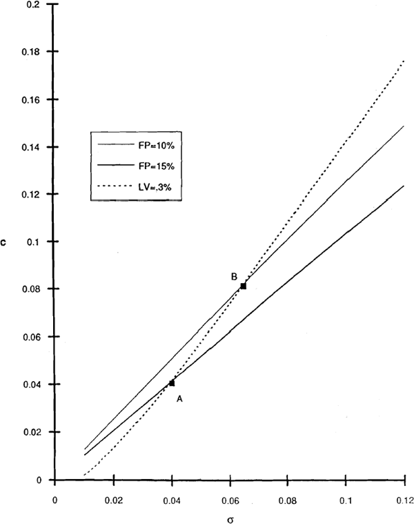
Figure 5 illustrates the potential conflict. Suppose that regulators pursue a goal of holding LV constant at 0.3%. As shown above, under an LV standard banks will be pushed toward positions of lower asset risk and lower capital ratios; in terms of Figure 5, they choose a point such as A rather than B. Although both points are on the same LV locus and hence lead to identical liabilities for the guarantor, the probability of bank failure is higher at A than at B. Similar conclusions follow if regulators pursue a constant-FP goal. The high-risk, high-capital portfolio chosen under an FP rule is on a higher LV locus than the lower-risk portfolios the bank could choose.

It follows that additional restrictions may be desirable under either type of rule. Under an LV rule a minimum ratio of equity to total assets may be needed to prevent failure probabilities from being pushed to unacceptable levels. Similarly, under an FP rule restrictions on the range of permissible assets and activities — perhaps in the form of limits on holdings of certain types of assets — may be necessary to set a maximum on σ and thereby limit the deposit guarantor's liability. Both of these types of supplemental restrictions (leverage ratios and portfolio limits) are already part of the regulatory structure in many countries; our results provide a rationale for their continued use even under comprehensive risk-based capital standards.

Footnotes

In fact, FP may be increasing or decreasing in σ, since for sufficiently insolvent banks the probability of failure is reduced by an increase in asset risk. A sufficient condition for ∂FP/∂σ to be positive is x < 0, which is satisfied when 0 < c < 1. We will restrict our attention to solvent banks, for whom this requirement is always met. [4]

The useful fact that 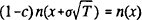makes this relationship between the slopes obvious. We consider only solvent banks, implying that x<0; the inequality holds for −8.64<x<0. Figure 3 graphs the combinations of σ and c that yield x=−8.64. [5]

Furlong and Keeley (1989) discuss the relative merits of modelling bank capital choices with the value of assets constant versus deposits constant within a contingent claim model. They conclude that a stronger logical case can be made for holding assets fixed and allowing deposits to vary. [6]

Since the bank's indifference curves reflect the total value of the deposit guarantee rather than the value per dollar of deposits, they do not coincide with the constant-LV loci. [7]

In practice, banks probably would not seek corner solutions. Contrary to the assumptions of the model, the total value of bank assets is not completely independent of risk. Risky lending is likely to be a source of economic rents for the bank, so that the optimal σ never would be zero. In addition, liquidity considerations probably require a non-zero proportion invested in riskless assets, limiting σ on the upper end. Under such conditions, an interior solution for σ and c probably would exist, and the bank would not jump to either extreme. Gennotte and Pyle (1991) develop a model in this spirit, in which the value of bank assets depends on σ. We do not incorporate this dependence explicitly in our model; under reasonable assumptions about functional forms, it would likely alter the magnitude but not the direction of the effects of risk-based capital standards. [8]