RDP 9204: The Term Structure of Interest Rates, Real Activity and Inflation 2. Theory

Standard Keynesian models typically have a single interest-bearing financial asset. The interest rate on this asset affects both the demand for money and investment. In order to examine the relationship between the yield curve and future changes in output a second asset must be introduced. This is done below in the context of a model in the IS-LM tradition with output being demand determined and prices adjusting slowly to their equilibrium value. It is similar in spirit to the model developed by Blanchard (1981); however it differs in that it allows investment to depend upon the real interest rate and does not consider the return on equities.

Investors are assumed to be able to invest in both a long and a short bond. The short bond is an instantaneous asset which cannot be traded across time while the long bond can be traded across time. With investors assumed to be risk neutral and having rational expectations, the relationship between yields on the short and long bonds is determined by the expectations theory of the term structure of interest rates. That is, the expected returns on short and long bonds are identical.

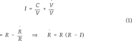
For simplicity assume the long bond is a consol paying interest (C) each instant with its price V = C/R, where R is the current market interest rate on the consol. The return from investing in the long bond consists of two parts; the interest payment (C) and the expected capital gain/loss . Given risk neutrality, the return on the long bond must equal the real return on the short term bond (I). That is,

This relationship between the interest rates on long and short bonds should hold in both nominal and real terms. As is standard, the nominal short rate (i) is equal to the real rate plus the forecast of the rate of inflation where the forecast is the rational expectations forecast :

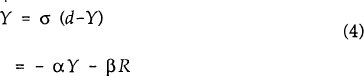
Goods market equilibrium occurs when aggregate demand equals aggregate supply. Aggregate demand is assumed to be a function of current income (Y) and the long real interest rate and is given by:

Output is assumed to adjust to demand over time according to the following^[1]:

Following the standard convention, the demand for real money balances is a function of current income and the current nominal short term interest rate:

Money is assumed to be exogenous and under the complete control of the monetary authorities.

In this model, if prices are completely flexible, changes in the money stock have no real effect on the economy as prices adjust instantaneously keeping real balances constant. However, it is assumed that while, in the long run, prices do adjust one for one with changes in the money stock, they do so only slowly. This allows monetary policy to have real effects on output in the short run. The following simple price adjustment mechanism is assumed:

where is the price level associated with equilibrium output and the level of nominal money .

First consider the extreme case in which θ equals zero (i.e. prices are fixed). In this case the system is defined by equations (1), (4) and (5). To find the steady state values of output and the long bond rate set and to zero and solve, obtaining:

As in the basic fixed price IS-LM model, monetary expansions increase output and reduce interest rates.

The dynamics of the system are derived in Appendix 2 and are summarised in Figure 1 which presents the phase diagram. Given the assumptions made about the signs of the parameters, the system exhibits a “saddle-path” shown by SS. Consider the effects of a monetary expansion. The R locus is shifted to the right increasing steady state output from to and reducing both the short and long steady state interest rates from to . The mechanism is standard. With fixed prices, higher real money balances force down the interest rate which in turn increases aggregate demand.

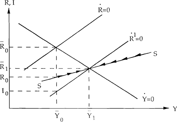
During the adjustment phase the equations of motion for R and Y are given by:

where ψ is speed of adjustment given by the negative eigen value. At any point in time the values of Y and R are read off the saddle path while the short rate is read off the locus. How then does the term structure of interest rates react to the monetary expansion? The short interest rate falls immediately (to I₀) due to the liquidity effect. Rational investors realise that in the medium/long run output will rise, increasing the demand for money. The short term interest rate must thus be expected to rise over time. As a consequence the long interest rate does not fall by as much as the short rate. In fact it falls to R₀ and then increases along the saddle-path towards the new equilibrium. Thus the yield curve initially becomes upward sloping in response to the monetary expansion and given rational expectations this upward slope of the curve is positively correlated with future increases in output. The speed of adjustment to the steady state is faster the larger are α, β and k.

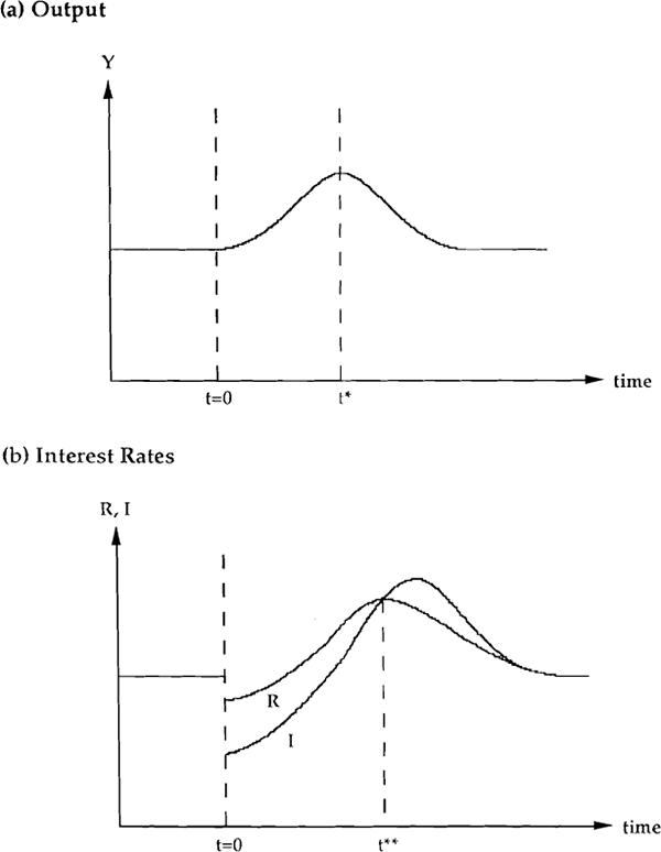
Now consider the case in which prices adjust slowly. In the long run, real money balances do not change in response to an increase in the money supply. Consequently, steady state real interest rates and output do not change in response to the monetary expansion. However, as prices are sticky there are short run effects. The adjustment paths towards the new steady state are derived in Appendix 2 and are given by equations (A18), (A19) and (A20). The equations of motion for and are functions of two declining exponentials. This implies that there is at most a single extreme point in their adjustment paths. Output is thus above its equilibrium level at all points through the adjustment phase and does not cycle around the new equilibrium. The long interest rate after falling initially, due to the liquidity effect, increases and overshoots its new equilibrium level. Declining output and the attendant fall in money demand and short rates then causes the long bond rate to fall. Stylised adjustments paths for output and the interest rates are given in Figures 2a and 2b. Once again a positively sloped yield curve predicts future increases in output. However, in contrast to the fixed price model, the increases in output are not permanent.

The above model focuses on shifts in the money supply. One frequent explanation for the shape of the yield curve is that in the future the rate of growth in the money supply is expected to change, altering expected future inflation. Such rate of growth shocks are analytically difficult to deal with in this type of model. Nevertheless, the general structure can be usefully employed to think about the effect of higher inflation expected some time in the future. It is clear that changes in the future expected rate of inflation should not affect the current short term interest rate as this rate is determined by instantaneous equilibrium in the money market. In contrast, the long bond is a forward looking asset whose price cannot jump when inflation actually moves to its new higher expected level. Thus, the price of the long bond must fall at the time that agents first expect higher inflation in the future. Following this fall, the yield on the long bond is higher than that on the short bond. The arbitrage condition requires that the price of the long bond must be expected to fall during the period preceding the future increase in inflation. As a result, higher expected future inflation must cause an initial jump in the interest rate on the long bond followed by further increases. With the short rate fixed, at least for the interim period, the yield curve steepens. With the assumption of some stickiness in prices, this upward slope will once again predict increases in output in the medium term. The issue of to what extent nominal interest rates reflect inflationary expectations is taken up in more detail in Section 4.

The above discussion attributes the ability of the slope of the yield curve to predict real activity to monetary policy. While real business cycle theory would generally eschew such an interpretation, it has difficulty explaining the forecasting success of the yield curve. Notwithstanding this difficulty, it is possible, by moving outside the strict real business cycle framework, to explain the forecasting ability with real shocks. In the above model the long term real interest rate and its time path are tied down by an arbitrage condition. Suppose instead that the long real interest rate is tied down by the marginal productivity of capital and that the short interest rate is determined in the money market. A permanent increase in the marginal productivity of capital would increase the long bond rate. Assuming that output increases only slowly in response to the productivity improvement, the demand for money increases only slowly. This gradually forces up the short term interest rate. In this world the initial increase in the yield spread correctly predicts future increases in output. The predictive power of the yield curve is thus not necessarily inconsistent with a real side explanation^[2].

This real side explanation suggests that a positively sloped yield curve predicts higher output at all future horizons. This is in contrast to the monetary model with flexible prices (in the long run) which suggests that the slope of the yield curve should have little predictive ability for changes in output between today and some distant point in time. The empirical evidence presented below and in Estrella and Hardouvelis (1991) suggests that the yield curve has no predictive power for cumulative output changes over horizons longer than three years. This supports the hypothesis that the predictive ability of the yield curves works primarily through the monetary channel.

Footnotes

This equation can be justified by arguing that spending adjusts slowly to its underlying determinants or alternatively that spending equals its underlying determinants but that firms respond to changes in demand by drawing down inventories and then increasing output. [1]

The real business cycle models, in the tradition of Kydland and Prescott (1988), have only a single interest rate. This rate is determined by the current and expected future marginal productivity of capital. The model is capable of generating predictions concerning the correlation between interest rates and output changes but does not address the question of the slope of the yield curve. [2]