RDP 8902: Option Prices and Implied Volatilities: An Empirical Analysis 5. Further Results on Pricing Discrepancies
May 1989
- Download the Paper 537KB
It has been pointed out that results of the kind reported in section 4 are necessarily conditional on the assumed option pricing model; rejection of the joint null hypothesis might, therefore, indicate rejection of the Black-Scholes model rather than rejection of forecast efficiency. This section considers two additional pieces of evidence which may have a bearing on this question. The first uses the fact that when the Black-Scholes assumptions are violated, the bias in the formula will be related to the extent to which the option being priced is in or out of the money; the formula tends to overvalue deep in-the-money options and to undervalue those which are deep out-of-the-money (see for example, Merton (1976)). Thus, if the apparent pricing biases detected in section 4 are caused partially by deviations from the Black-Scholes assumptions, we would expect the empirical biases to be correlated with the option deltas, which can be used as a measure of the extent to which an option is in or out of the money.
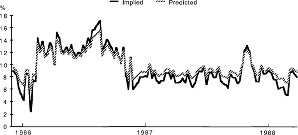
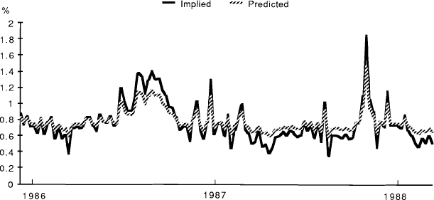
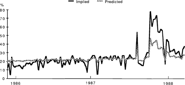
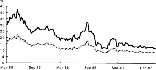
Estimated pricing biases can be obtained by using fitted values for expected volatility from equations (6) and (8b) to obtain a time series of estimated option values, which can then be compared with observed prices. A comparison between the estimated volatilities and those implied in the option prices appears in Figures 1 to 4. Generally speaking, these imply price discrepancies which vary in a range between zero and about 30 per cent. (For the SPI options the calculations, though performed for the full sample, are based on the estimated pre-crash relationship.) The graphs also illustrate the general point that “fitted” volatilities tend to be less variable than those implied in actual option prices. The currency options case differs from the other three in that there is also an apparent unidirectional bias in levels, with implied volatilities always exceeding those predicted by the forecasting equation. However, the gap narrows through the sample period, perhaps reflecting an increasing competitiveness in the pricing of these options.
IMPLIED AND PREDICTED VOLATILITIES


The proposition that the pricing biases are related to the options' deltas is tested using simple linear regressions of the calculated biases against the relevant series of deltas. (This is not applicable to the case of currency options, since all the currency options in the data set are at-the-money.) Results for these regressions are reported in Table 5. They show quite clearly a lack of any significant correlation between these variables; estimated pricing biases appear not to be correlated with the extent to which options are close to the money. This provides one piece of evidence that our results are unlikely to be explained as being due to deviations from the Black-Scholes assumptions.
| Dependent variable Price bias on: |
Constant |
Option Delta |
R2 |
dw |
|---|---|---|---|---|
| Bonds calls | 0.09 (4.19) |
−0.006 (−0.30) |
0.50 |
1.05 |
| puts | 0.16 (4.62) |
0.04 (1.13) |
0.15 |
0.95 |
| Bills calls | 0.12 (4.01) |
0.06 (2.11) |
0.12 |
1.38 |
| puts | 0.16 (7.18) |
−0.02 (−1.04) |
0.24 |
1.04 |
| SPI calls | 0.12 (2.38) |
0.11 (1.64) |
0.32 |
1.84 |
| puts | 0.07 (2.38) |
0.04 (1.31) |
0.26 |
0.92 |
Note: t – statistics in parentheses. |
||||
As a second piece of evidence, which has a direct bearing on market efficiency, it may be asked whether use of statistically efficient forecasts implied by use of equations (6) and (8b) would have led to significant excess returns within the sample period. (At a later date it is hoped to repeat this exercise using out of sample data.) To investigate this question the comparison between actual and estimated option prices described above was used to simulate the following hedged trading rule:
buy any option that is undervalued and hold to expiry;
sell any option that is overvalued, and hold the position to expiry;
in each case, delta hedge the initial position in the underlying instrument, but with no subsequent rebalancing.
The delta is evaluated using fitted volatilities.
The realised excess return on a hedged call transaction under this rule is then given by:
| where | D | = | 1 for a buy |
| = | −1 for a sell |
Put returns are defined analogously.
Within sample returns calculated in this way are summarised in Table 6.
| Calls | Puts | |
|---|---|---|
| Bonds | 58 | 57 |
| Bills | 70 | 76 |
| SPI | 54 | 51 |
| Currency | 77 | 80 |
Note: The table shows the percentage of observations in the sample showing excess returns as defined by equation (10). |
||
The most dramatic results are those for bill futures options, and currency options. In both these cases roughly three-quarters of the observations generate positive excess returns within sample. The currency option results are generated mainly by an implicit overpricing during the sample period; since forecast volatilities were always less than those implied in option prices, the trading rule given by equation (9) indicated a sell in every period. For bond and SPI options the figures for excess returns are smaller at around 60 per cent for bonds, while for the SPI, it is barely above the 50 per cent which one would expect to obtain randomly. This perhaps confirms some of the reservations which were expressed in the earlier discussion of the SPI results. For the remainder, however, the results provide some support for the view that expectations errors, rather than biases in the pricing formula, are responsible for the anomalies reported in section 4. In this regard, it is worth noting that the rule used to detect excess returns here was a particularly unsophisticated one. Outstanding options were not assumed to be delta hedged to maturity, and there was no attempt to weight the size of each trade according to the relative extent of each overvaluation or undervaluation. If anything, such a trading rule would be likely to understate the presence of excess returns in the sample.
