RDP 8703: Money Demand, Own Interest Rates and Deregulation 2. The Stability of Money Demand
May 1987
- Download the Paper 1.1MB
Previous studies of money demand in Australia do not include data affected by deregulation in the mid 1980s. Only recently has sufficient data come to hand t test whether the old relationships have been robust to the changes. The starting point for the present study is a paper by Stevens, Thorp and Anderson (1986), which re-estimates functional forms used in earlier literature on money demand functions.
Four representative studies of money demand in Australia were selected by Stevens et. al. These were replicated and updated with the purpose of assessing their stability over original and extended sample periods. Three M3 equations and one M1 equation were subjected to a variety of stability tests. The M3 equations estimated were those of Sharpe and Volker (1977), Porter (1979) and Freeland (1984). All three used primarily double log, Koyck adjustment formulations with the real money stock explained by gross domestic product and interest rates. Pagan and Volker (1981) estimated a more general equation for M1.
All the earlier demand functions for M3 were found by Stevens et. al. to break down when updated to early 1986. This may have resulted from the effects of deregulation, or errors in the specification of the original equations. This was less clear for the Pagan and Volker M1 equation. There is no earlier literature for the relatively new BM aggregate.
A different methodology is applied in this paper to assess the stability of money demand. We begin with a general formulation of a money demand function, and the impose parameter restrictions accepted by the data to obtain preferred specifications. These are then subjected to stability tests over the sample period.
A single equation approach is adopted in line with previous Australian and international literature in this area. In principle, both the money supply and demand processes could be modelled in a full system context, particularly if one is interested in examining monetary policy transmission mechanisms. This ensures simultaneity problems are fully accounted for.[1] The aim of this paper is more limited. It attempts to examine the nature of relationships between money income and interest rates over the recent period of deregulation, using some new data for own rates of interest on holding money balances. The sample period is relatively short, and the focus is on how the simple relationships behave as deregulation impacts on both competing and own rates of interest.
Following previous studies we postulate a long-run equilibrium relationship of the form:
where M is money, P the price level (GNE deflator), xi (i = 1,..... i) are
other variables, αi (i = 0...... I) are parameters, and lower case letters denote logarithms. The general form of the short-run dynamic analogue to equation 1 in distributed lag form is:
Demand functions of this general form were estimated on quarterly data over the sample period 1974Q2 to 1986Q2 for M1, and 1977Q1 to 1986Q2 for M3 and BM.[2] The independent variables were real income, Y, the two-year government bond rate, R, and constructed own interest rates for M3 and BM, RM3 and RBM.[3] Details of the data are supplied in Appendix C.
An important part of the Bank's recent empirical research motivating the present study has been the construction of own interest rates for M3 by Evans (1986), and the updating of this work and construction of a BM own rate by Thorp (1986).[4] Own interest rates must be included with the competing rates to measure the opportunity cost of holding money. Furthermore, while other rates may also be important, the rate of return available on a broader definition of money is likely to be the most relevant competing rate for narrower definitions. Thus, the M3 own rate is an important aspect of the opportunity cost of holding current deposits. Similarly, rates available from financial institutions outside of the banking system may be the most relevant competing rate for bank deposits.
The specification of the opportunity cost argument was also carefully tested, along with the relevant lag structure. Results are reported in full for M1, M3 and BM (for the case of J=1) in Tables 1, 2 and 3, respectively.[5]
| Restrictions | β0 | β10 | β11 | β20 | β21 | γ1 | γ2 | F test of restric. |
Critical Value 5% |
Fit | h | |
|---|---|---|---|---|---|---|---|---|---|---|---|---|
| 1. | Unrestricted |
−0.606 (−0.556) |
0.485 (2.868) |
−0.232 (−1.26) |
−3.378 (−2.753) |
1.724 (1.339) |
−0.251 (−1.555) |
0.045 (0.379) |
– |
– |
 |
undefined |
| 2. | γ2 = 0 |
−0.458 (−0.455) |
0.478 (2.875) |
−0.238 (−1.314) |
−3.317 (−2.757) |
1.751 (1.377) |
−0.204 (−1.993) |
0.00 |
0.144 |
4.08 |
 |
−0.161 |
| 3. | γ2 =0 β11 = 0 |
−0.507 (−0.499) |
0.275 (4.462) |
0.00 |
−3.39 (−2.795) |
1.618 (1.266) |
−0.233 (−2.304) |
0.00 |
0.917 |
3.23 |
 |
0.218 |
| 4.* | γ2 = 0 β11 = 0 β21 = 0 |
0.22 (0.27) |
0.289 (4.739) |
0.00 |
−1.93 (−5.09) |
0.00 |
−0.324 (−4.576) |
0.00 |
1.143 |
2.84 |
 RMSEb =0.029 |
0.097 |
| 5. | γ2 = 0 β11 = 0 β20 = 0 |
1.354 (0.634) |
0.264 (3.981) |
0.00 |
0.00 |
−1.779 (−4.151) |
−0.416 (−5.027) |
0.00 |
3.205 |
2.84 |
 |
−0.145 |
|
Note: (a) t statistics in parenthesis. |
||||||||||||
| Restrictions | β0 | β10 | β11 | β20 | β21 | γ1 | γ2 | F test of restric. |
Critical Value 5% |
Fit | h | |
|---|---|---|---|---|---|---|---|---|---|---|---|---|
| 1. | Unrestricted |
−0.750 (−1.772) |
0.384 (3.099) |
−0.115 (−0.764) |
−4.785 (−2.268) |
2.941 (1.441) |
−0.222 (−1.140) |
0.036 (0.212) |
– |
– |
 |
undefined |
| 2. | γ2 = 0 |
−0.717 (−1.852) |
0.380 (3.161) |
−0.113 (−0.765) |
−4.840 (−2.350) |
3.032 (1.545) |
−0.187 (−1.818) |
0.00 |
0.045 |
4.20 |
 |
−0.582 |
| 3. | γ2 = 0 β11 = 0 |
−0.740 (−1.929) |
0.317 (3.641) |
0.00 |
−5.184 (−2.597) |
3.009 (1.544) |
−0.232 (−2.758) |
0.00 |
0.306 |
3.34 |
 |
−0.303 |
| 4.* | γ2 = 0 β11 = 0 β21 = 0 |
−0.797 (−2.043) |
0.329 (3.712) |
0.00 |
−2.375 (−2.824) |
0.00 |
−0.237 (−2.769) |
0.00 |
0.962 |
2.95 |
 RMSEb =0.014 |
−0.087 |
| 5. | γ2 = 0 β11 = 0 β20 = 0 |
−0.706 (−1.694) |
0.287 (3.055) |
0.00 |
0.00 |
−1.601 (−1.831) |
−0.207 (−2.275) |
0.00 |
2.347 |
2.95 |
 |
−0.097 |
|
Note: (a) t statistics in parenthesis. |
||||||||||||
| Restrictions | β0 | β10 | β11 | β20 | β21 | γ1 | γ2 | F test of restric. |
Critical Value 5% |
Fit | h | |
|---|---|---|---|---|---|---|---|---|---|---|---|---|
| 1. | Unrestricted |
−0.416 (−1.037) |
0.282 (2.610) |
−0.193 (−1.576) |
0.623 (1.886) |
−0.857 (−2.471) |
−0.281 (−1.599) |
0.237 (1.581) |
– |
– |
 |
Undefined |
| 2. | γ2 = 0 |
−0.432 (−1.052) |
0.293 (2.644) |
−0.195 (−1.558) |
0.594 (1.755) |
−0.881 (−2.482) |
−0.050 (−0.500) |
0.00 |
2.50 |
4.20 |
 |
−1.053 |
| 3. | γ2 = 0 β11 = 0 |
−0.773 (−2.171) |
0.240 (2.226) |
0.00 |
0.500 (1.467) |
−0.869 (−2.395) |
−0.150 (−1.8921) |
0.00 |
2.53 |
3.34 |
 |
−0.220 |
| 4. | γ2 = 0 β11 = 0 β21 = 0 |
−0.769 (−2.010) |
0.309 (2.762) |
0.00 |
−0.057 (−0.213) |
0.00 |
−0.215 (−2.683) |
0.00 |
3.79 |
2.95 |
 |
−0.780 |
| 5.* | γ2 = 0 β11 = 0 β20 = 0 |
−0.889 (−2.514) |
0.289 (2.764) |
0.00 |
0.00 |
−0.506 (−1.872) |
−0.185 (−2.392) |
0.00 |
2.47 |
2.95 |
 RMSEb 0.014 |
−0.217 |
|
Note: (a) t statistics in parenthesis. |
||||||||||||
(a) Money demand estimates
The coefficients on the second lag of real money balances were insignificantly different from zero for all three aggregates, and F tests confirm that the restriction γ2=0 is accepted by the data. Restrictions on the income terms were also similar between the aggregates. However, the way in which interest rates enter the equations differs between BM and the other aggregates.
Consider first the interest rate terms. Collinearity problems preclude the inclusion of a spectrum of rates. For M1 the main competing rate was found to be the rate of interest on M3.[6] Exclusion of the lagged interest rate (β21=0) was accepted by the data, while excluding the current rate was not. For M3, the main competing rate was found to be that available on broad money. The M3 own rate was also significant, and the restriction of equal and opposite signs on the two rates was accepted by the data. Again, it was the contemporaneous opportunity cost that was included in the equation.
For BM, the competing rate is the two-year government bond rate. The differential between the competing and own rates was again included in the equation. As with M3, the restriction of equal and opposite signs on the competing and own interest rates was accepted. However, restricting the parameter β20 on the current interest rate differential to zero was accepted by the data, whereas excluding the lagged term is not. This finding contrasts strongly with that for M1 and M3. The evidence suggests the absence of a contemporaneous impact of interest on broad money demand.
The long-run semi-elasticities of money demand with respect to interest rates are shown in Table 4. It is interesting that these are high for M1 and for M3, but markedly smaller for BM.
| M1 | M3 | BM | |
|---|---|---|---|
| Income elasticity | 0.89 | 1.39 | 1.56 |
| Interest rate semi-elasticity | −5.96 | −10.02 | −2.74 |
| Mean lag (quarters) | 3.09 | 4.83 | 5.41 |
With regard to the income terms, the coefficient β11 on lagged income is constrained to zero for all three aggregates. The long-run income elasticities of money demand implied by estimates of β10 are also shown in Table 4. As the aggregate becomes broader, the income elasticity tends to rise. This is consistent with the role of money as a store of wealth in the case of the broader aggregates.
Also shown in Table 4 are the estimated mean lags. These are short for the narrow transactions aggregate M1, but lengthen somewhat for M3 and again for BM. Transactions costs associated with shifting between interest bearing deposits and/or less liquid government bonds would be consistent with this finding.
(b) Stability tests
The preferred money demand equations (shown with an asterisk in each of Tables 1 to 3) were subjected to stability tests. Particular attention was given to the 1980s. Recursive regression (cusum and cusum of squares) and moving regression (homogeneity statistic) tests were used. Quandt's likelihood ratio helped identify potential periods of structural breaks in the data generating process. The significance of the potential break in the data associated with the global minimum of Quandt's likelihood ratio was subjected to a Chow or F test. A Chow test was also conducted for 1985Q1, the quarter in which monetary targeting was suspended because of the impact of deregulation. The main findings are summarised in Table 5; more detailed results are set out in Appendix B. Appendix A explains the test procedures in full.
| Test | Equation | ||
|---|---|---|---|
| M1 | M3 | BM | |
| Cusum | |||
| – forward | – | – | – |
| – backward | – | – | – |
| Cusum of Squares | |||
| – forward | * | ** | * |
| – backward | – | – | – |
| Moving Regression Homogeneity (at largest sample size) | – | – | – |
| Chow Test | |||
| – 1985 Q1 | * | ** | * |
| – Min Quandt | ** | ** | – |
|
Notes: An ** denotes rejection of the null hypothesis of stability at the 1 per cent level. An * indicates rejection at the 5 per cent level. |
|||
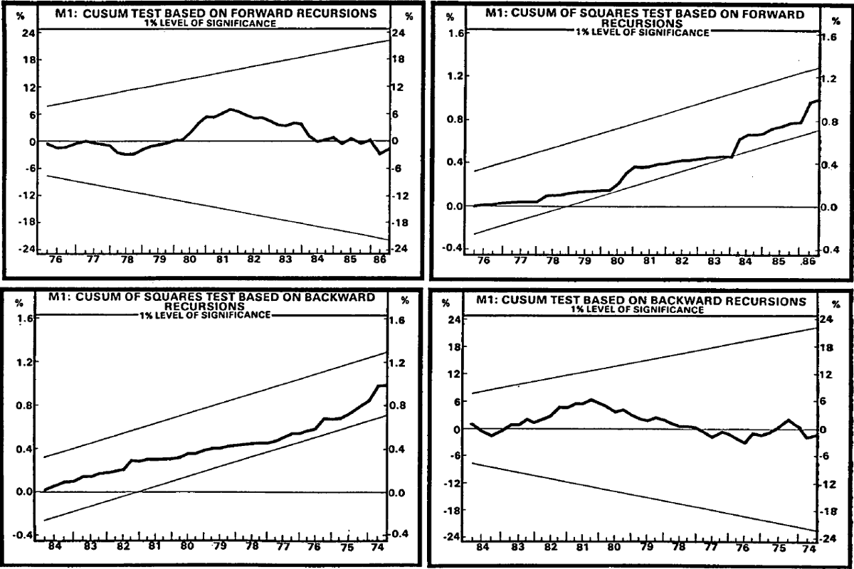
The M1 equation shows some evidence of instability under the procedures adopted. The equation seems reasonably stable on the basis of the Brown, Durbin and Evans (1975) tests (see Chart 2), with the possible exception of the forward cusum of squares case. However, the Chow test based on the break point identified by the minimum of Quandt's likelihood ratio was significant even at the less demanding 1 per cent level. This occurs in 1979. At this time, there was a shift in monetary policy operating procedures, with the introduction of the Treasury note tender system. The level of cash in the economy was less influenced by fluctuations in the budget deficit than had previously been the case.
The M3 equation shows even more distinct signs of instability during the 1980s. The smallness of the sample size suggests that particular care should be taken in interpreting the results. Nevertheless, the normalised cumulative sum of squared recursive regression residuals move outside of the significance bounds during the early 1980s, even at the 1 per cent level, as is shown in Chart 3.
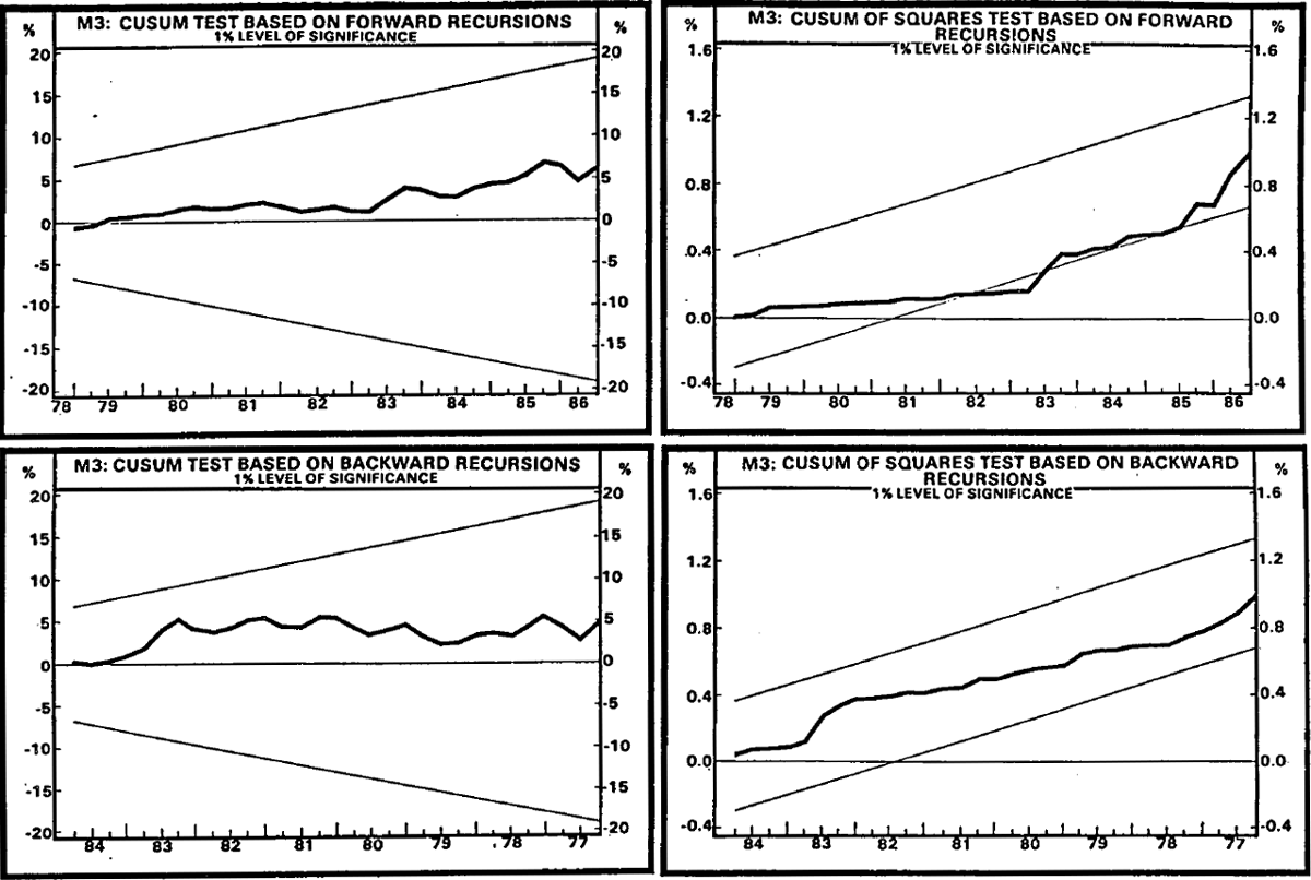
The official M3 projection was suspended in early 1985 mainly because of distortions associated with deregulation. A Chow test confirms that this break is significant even at the 1 per cent level. This result offers some support for the judgement made at that time. Similarly, a Chow test confirms rejection of the null hypothesis of stability for the break point identified by the minimum of Quandt's likelihood ratio (1983Q1).
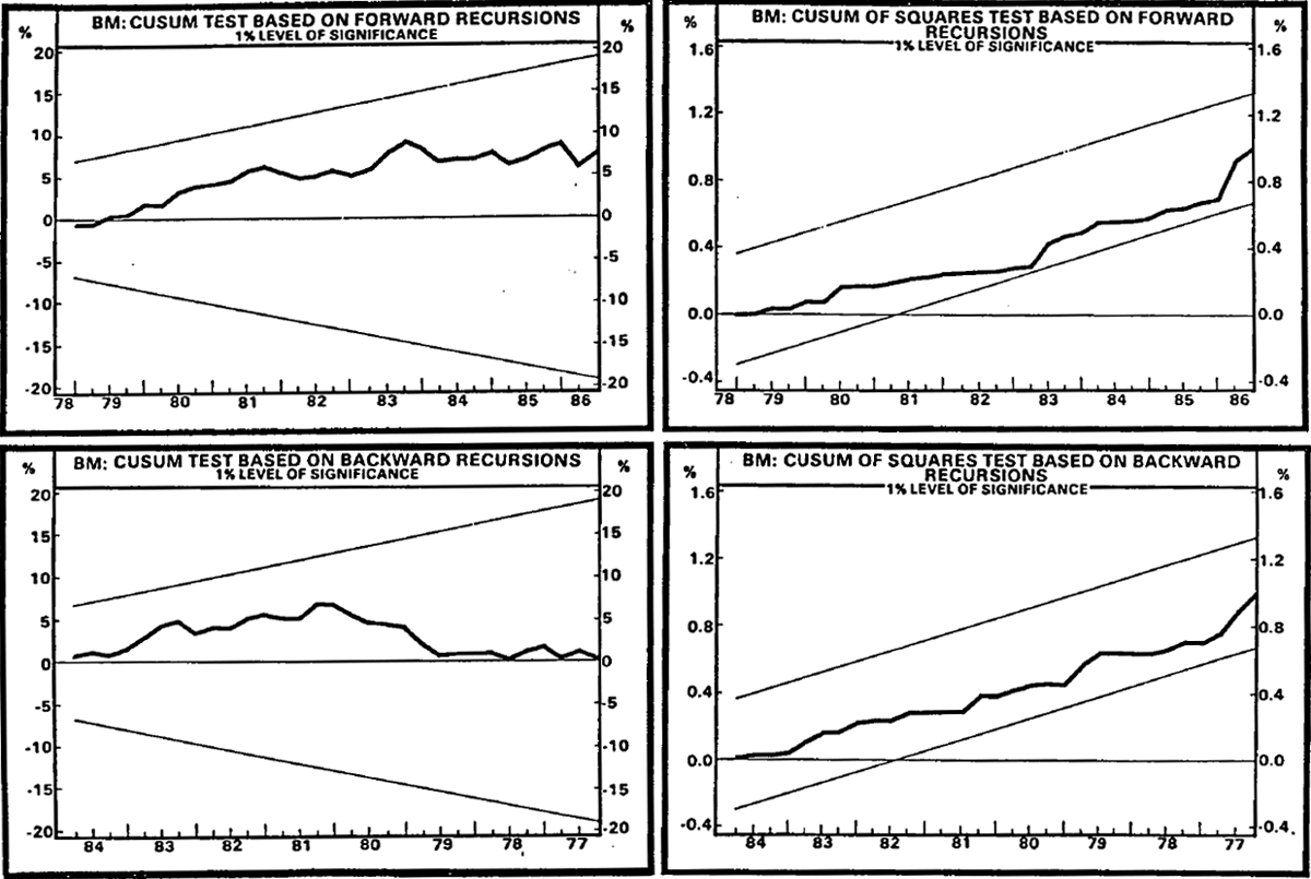
The results for the relatively new BM aggregate also provide an interesting contrast (see Chart 4). While also being qualified by the small sample size, the initial findings are relatively encouraging. The null hypothesis of stability cannot be rejected at the 1 per cent level for all of the tests conducted. At the 5 per cent level there are very marginal rejections by the forward cusum of squares test and the Chow test at 1985Q1.
(c) Interpreting deregulation
A period of financial deregulation impacts on monetary aggregates through four main channels:[7]
- movements in relative interest rates;
- measurement of the aggregates;
- measurement of the relative pecuniary costs and non-pecuniary returns on holding money; and
- changes in money holdings for precautionary motives.
Deregulation affects relative interest rates. For example, banks are now permitted to set market interest rates on all deposits. Maturity controls which previously prevented banks from paying interest on current deposits and from competing for call funds were removed in August 1984 and April 1985. Chart 5 shows the main relative interest rates used in this paper: the own rate of interest on M3, which acts as a proxy for the opportunity cost argument for M1; the BM own rate minus the M3 own rate, which acts as the opportunity cost for M3; and the bond rate minus the BM own rate, which is the opportunity cost variable for BM. The bond rate is also shown on its own, as an indicator of the stance of monetary policy. Its upward trend reflects higher inflation during the 1970s, with peaks during periods of monetary restriction, most notably early 1982 and late 1985.
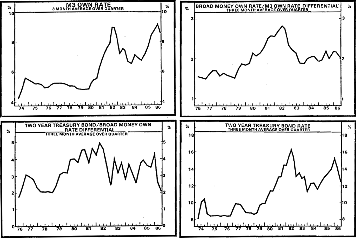
The opportunity cost for M1 (the rate on M3) was flat until the early 1980s. The impact of deregulation on the rate is apparent. Its rises and falls go some way towards explaining the fluctuations in M1 during the 1980s shown in Chart 1.
The opportunity cost for M3 (the differential between the BM rate and the M3 own rate) fluctuates within a range of 1–1/2 to 3 percentage points, while that for BM (the bond rate minus the BM own rate) lies within a range of 2 to 5 percentage points. Prior to deregulation, the M3 own rate was less able to keep pace with the competing rate during periods of monetary restriction in 1981 and 1982. This gives rise to a distinct peak, which is not repeated in 1985 when monetary policy was tight but financial markets were fully deregulated. While the differential between the bond rate and the rate on BM is more volatile, it has a distinctly flatter profile. Non-bank financial institutions included in broad money were better placed to compete in financial markets during periods of monetary restriction.
To the extent that these relative interest rate arguments are appropriate, they provide some explanation for recent patterns in monetary growth. The marked slowdown in the growth of M1, for example, is explained in part by the high level of competing interest rates during 1982 and 1985, which are not offset by any significant own rate effect. However, one has to be a little sanguine about the relative stability of the M1 equation. The impact of deregulation may have been of a compensatory nature specific to the period under consideration. For example, improved services and reduced costs implied by automatic teller machines and point of sale electronic funds transfer (EFT) could have increased the use of currency and reduced reliance on cheques. The ratio of currency to current deposits has risen over the past couple of years. If competition from non-bank financial intermediaries has also just kept pace with banks in providing these services, the appearance of relative stability in the aggregate relationships may be cosmetic.
The failure of the own rate of interest on M3 to match interest rates on deposits with financial institutions other than banks in the late 1970s and early 1980s helps explain the slow growth of M3 relative to BM until 1982. The late 1970s and early 1980s were associated with increased intermediation by non-bank financial institutions at the expense of banks. The subsequent sharp narrowing of the differential after the middle of 1982 by a full percentage point, helps explain the faster growth of M3 compared to BM, even as monetary restriction gathered pace in 1985. These movements in relative yields help explain the process of disintermediation affecting M3 in the late 1970s and early 1980s, as well as the subsequent reintermediation after deregulation. However, despite the fact that relative interest rates explain a considerable proportion of the variability of M3, signs of econometric instability remain.
It is likely that this instability is related to the other three channels through which deregulation influences monetary aggregates: measurement of the aggregate; measurement of the pecuniary costs and non-pecuniary returns; and precautionary motives. If the appropriate measurement of an aggregate changes during the sample period, attempts to estimate a stable demand function would normally be frustrated. This typically occurs when new assets are created, such as banks offering deposit terms which compete more favourably with other financial institutions. Substitution towards these new bank assets will shift the demand function. The aggregate is simply not comparable before and after the changes.
The pecuniary costs and non-pecuniary returns on holding money are unobservable, and are treated as constant in empirical money demand functions. The introduction of automatic teller machines and EFT may greatly alter these costs and returns, causing money demand functions to shift. As specific variables to measure these costs cannot be included in the equation, the shifts will tend to be reflected in changes to the constant term during a period of deregulation.
It is also possible that precautionary motives for holding deposits may vary as competition within the financial system increases.
Evidence that the M3 equation is unstable does not distinguish effectively between these types of instability. The approach may, however, give some idea of the size of the overall impact of deregulation.
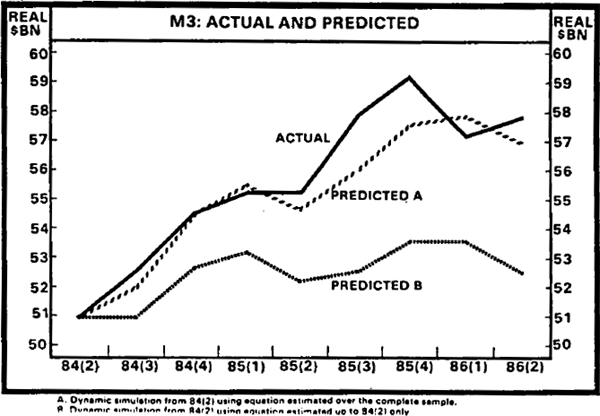
Chart 6 presents estimates of the size of the impact of deregulation and financial innovation on M3. It will be recalled that 1984Q2 was identified as a possible break in the data generating process. The equation estimated over the full sample period was dynamically simulated over the period 1984Q2 to 1986Q2. It predicts the actual pattern of M3 reasonably well. However, the same equation estimated to 1984Q2 underpredicts subsequent M3 developments. The gap between the two predictions gives an indication of the problems of interpreting M3 on the basis of relationships observed up to 1984. By 1986Q2 the gap between the two predictions is equivalent to 8 per cent of the money supply.
In contrast to M3, the BM equation is relatively stable. It is unlikely that movements in the differential between the bond rate and the own rate on BM before and after 1982 explain much of the behaviour shown in Chart 1. The differential is more volatile around a flatter trend throughout the period. Moreover, the interest semi-elasticity is smaller than for M1 or M3, no contemporaneous interest rate effect was identified, and the adjustment lag is noticeably longer than for the other aggregates. On the other hand, the income elasticity is relatively high. It is likely that the behaviour of broad money is much more closely tied to the pattern of economic activity.
Footnotes
This approach has been taken in the Bank's econometric model RBII. See, for example, Jonson and Trevor (1981), Jonson, McKibbin and Trevor (1982) and Fahrer, Rankin and Taylor (1984). [1]
The sample periods chosen are the longest possible given data constraints. For example, it was possible to construct the own rate for M3 only back to 1974. See Evans (1986). [2]
The construction of the own rate of interest for M3 and BM is discussed in Appendix D. [3]
As yet the importance of market interest rates on cheque accounts is not sufficient to warrant an own rate for M1. The practice of banks at present is far from uniform and the emergence of interest bearing current accounts mainly involves absorption of service charges rather than the provision of market rates of return. [4]
Tests were conducted for the case of J=3 and J=2. Zero restrictions on all variables subscripted j=2,3 were accepted at the 5 per cent level. Presentation of the results is greatly simplified if we restrict ourselves to the case of j=0,1. [5]
The M3 own rate was acceptable at a higher level of probability on the basis of t tests but, more importantly, the M1 equation proved more stable with this specification. [6]
Milbourne (1986) characterises the specific deregulatory changes according to three of these channels of influence. [7]


