RDP 8703: Money Demand, Own Interest Rates and Deregulation Appendix A: Statistical Tests

This appendix sets out in detail the stability tests applied to the preferred equations for M1, M3 and Broad Money recorded in Tables 1, 2 and 3. The tests are largely derived from Brown, Durbin and Evans (1975) who presented a group of formal significance tests for the constancy of estimated coefficients (β) and sample variance . Even though the tests are presented as formal significance tests, the authors recommend that they be regarded as “yardsticks” rather than conclusive decision rules.

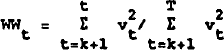
The CUSUM and CUSUMSQ plots use the recursive residuals of the regression to test the hypothesis of constant β and σ² over time.

The CUSUM of recursive residuals is defined as:

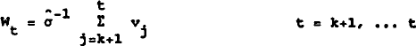
where k is the number of estimated parameters;

v_t is the recursive residual in period t, i.e.

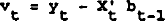
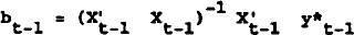
where b_t−1 is the OLS estimator based on the first t−1 observations, i.e.

and

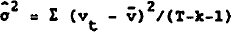
where is the arithmetic mean of the residuals.

The CUSUMSQ is

Under the null hypothesis of stability, the recursive residuals are uncorrelated, with zero mean and constant variance. This property is useful in interpreting plots of the CUSUM and CUSUMSQ: since the distributions of the statistics are known, boundary lines can be constructed around the mean value lines such that the probability of crossing the boundaries is equal to the chosen significance level of the tests.

The plots thus serve the double purpose of providing a formal hypothesis test for stability and giving a graphical representation of the residuals from which breaks in the data can sometimes be identified.

The CUSUM test is sensitive to a disproportionate number of residuals of the same sign, which moves the plot away from the mean value line. It is also useful for detecting structural breaks in the data, which appear as a secular increase or decrease in the plot.

The CUSUMSQ is more sensitive to haphazard changes in the residuals, and is also useful for detecting structural breaks and/or gradual increases in variances over time.

Quandt's log-likelihood ratio and the Chow test for structural break were used in tandem to detect potential breaks in the data. Quandt's log-likelihood ratio guides the choice of break point for the Chow test. The ratio is calculated for each t=r from r=k+l to r=T-k-l:

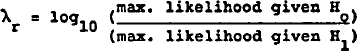
where H₁ is the hypothesis that the samples before and after r come from different populations.

The most likely point for structural break is at the point r where λ_ris minimised.

F tests and Chow tests were conducted at the minimum of λ_r for each of the preferred equations. The F statistic is calculated:

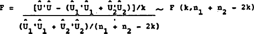
where n₁ is the sample from 1, .... r;

n₂ is the sample from r+1, …, T;

is the sum of squares of the least squares residuals over the entire sample. Subscripts 1 and 2 indicate the same statistic for each of the two sub-samples.

Where one sub-sample is too small to estimate a regression, the alternative Chow statistic is:

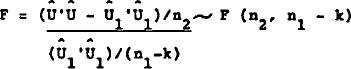
where n₁ is the largest of the two sub-samples.

The last of the stability tests used is Brown, Durbin and Evans' Homogeneity Statistic, which also tests for changes in estimated coefficients and sample variance. The Homogeneity statistic is calculated from the residual sums of squares of moving regressions of sample size n. The null hypothesis of constant β and is tested by the statistic:

where n is the length of the moving regression;

S(r,s) is the residual sum of squares of the regression calculated for observations r to s inclusive; p is the integral part of T/n; and k is the number of parameters.

Under the null hypothesis of stability the statistic is distributed as F(kp−k,T−T−kp).

Notice that all of the stability tests described above rely on an assumption of homoskedastic errors: they are joint tests of constant coefficients and sample variance. Tests tend towards rejection of the null of stability when heteroskedasticity is present. The results of the Breusch-Pagan test (reported in Appendix B) suggest the possibilty of heteroskedasticity for M3 and BM, although this test may be unreliable in such small samples.