RDP 8403: Modelling Recent Developments in Australian Asset Markets: Some Preliminary Results 5. Simulation Results

The version of RBII used as a basis for the construction of this simulation model is that described in detail in Fahrer, Rankin and Taylor (1984); the resulting simulation model is presented in summary in the Appendix to this paper.

A control solution was found for the modified model, using 1976(1) as a starting point and running for 28 quarters. In this solution, the target growth rate of money is set to a constant 0.025 per quarter, which was approximately the historical average over the period. This gives a specification for the money target variable in equation (13') of M_T = M₀ e^0.025t where M₀ is the actual value of the money supply at the start of the simulation, at which time t=0.

This control solution cannot be compared with the historical outcome, since the assumptions about market structures and policy determination did not apply over the period. It is possible, however, to examine the properties of the simulation model itself by analysing the deviations from the control solution caused by exogenous shocks of various kinds.

Three shocks are considered:

• a sustained 5 per cent increase in real current government spending (a non-accommodated fiscal expansion);
• as above, with an increase of 0.5 per cent per quarter in targeted monetary growth (an accommodated fiscal expansion); and
• as the first shock, with a decrease of 1.0 per cent in the long-run target value of real household saving (a non-accommodated fiscal expansion with increased consumer confidence).

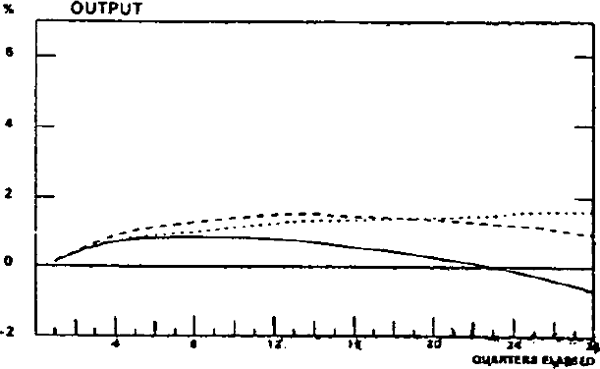
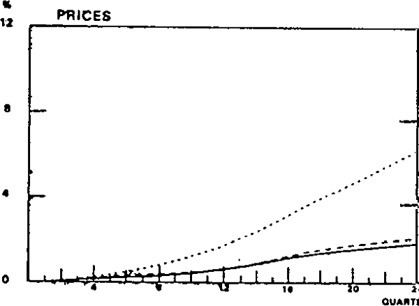
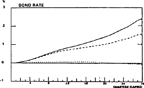
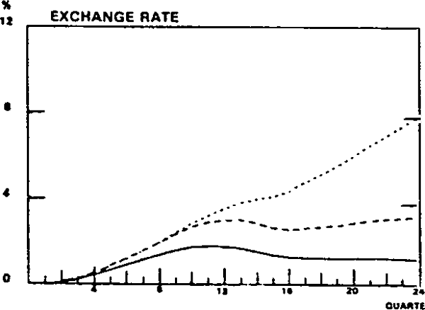
The effects of these shocks, in terms of deviations from the control solution, are shown for key variables in figures 1–7.

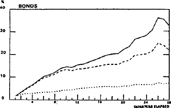
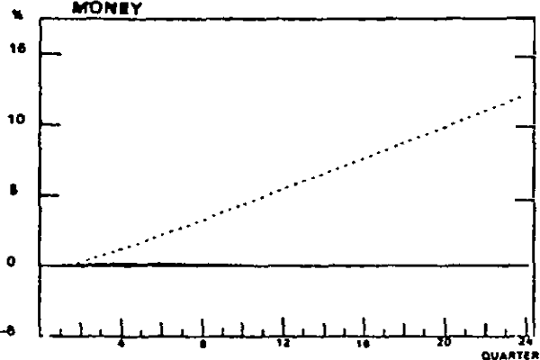
The degree of accommodation or non-accommodation in each case is clear from figures 3, 5 and 6. In the first and third cases, the money supply (figure 6) is held to within 0.2 per cent of control throughout the simulation period. Bonds (figure 5) rise strongly, as does the bond rate (figure 3). In the second case, the additional growth of money implies a path for bond sales which has the effect of stabilising the bond rate within 0.1 percentage points of its control value.

In all cases, it is monetary growth that is assumed to be targeted, and the results show that the assumed reaction function (13') keeps the money supply quite close to its specified target.

5(a). The case of non-accommodated fiscal expansion

This case is shown as the solid lines in the figures.

Output (figure 1) rises slowly, peaking after seven quarters and declining thereafter. The peak multiplier is approximately 0.97, and declines to zero after twenty-two quarters. This “crowding out” effect is due primarily to the large rise in interest rates produced by the bond-selling policy assumed but also because of the real appreciation that occurs towards the end of the simulation period, and the increase in the excess supply of inventories that is present throughout all but the first six quarters of the simulation.

The price level (figure 2) is permanently increased, though only slightly: on average, the annual inflation rate is about 0.3 percentage points higher than control, primarily due to rises in unit labour costs. It is slower at first, when most of the spending stimulus is reflected in output, but rises as the output multiplier declines.

The increased demand worsens the current account for six years. This is offset by capital inflow which is attracted by higher domestic interest rates and (for the first four years, while interest rates are rising slowly) by a real depreciation (a rise in EP_W/P) which generates an expectation of appreciation in the future. From the fifth year, with income declining and the current account improving, the exchange rate appreciates in real terms.^[11]

The stock of money is held to within 0.2 per cent of control throughout the simulation; this result shows closer monetary control than earlier versions of the model.^[12] With money being held at control, a large increase in bond sales (figure 5) is needed to finance: the budget deficit (via equation 13'). This increase in the supply of bonds leads to an increase in the bond rate (equation (20'); figure 3). By the end of the simulation period it is about 2.5 percentage points above control.

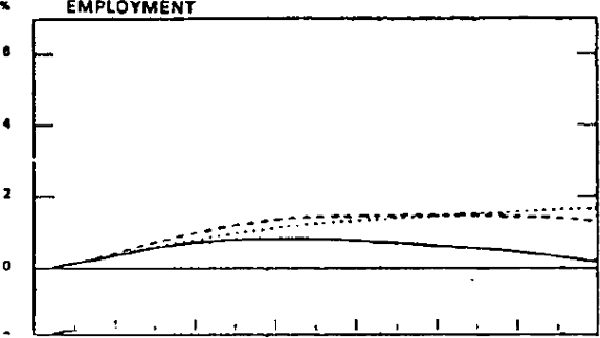
The response of employment is shown in figure 7. Real wages slightly rise at first, due to the pressure of higher activity, but begin to decline after eleven quarters. The initial rise in real wages prevents employment rising in line with output but as real wages fall employment is prevented from falling below control towards the end of the period. Variations in real wages are, therefore, an important factor in smoothing the employment effects of the cycle in real output in this simulation.

5(b). The case of accommodated fiscal expansion

The effects of the accommodated rise in government expenditure are shown by the short-dashed lines in the figures.

Output grows more quickly than under non-accommodating monetary policy, and levels out to approximately 1.61 per cent above control after seven years. (This implies a multiplier of about 1.88). This result is again conventional; the rise in interest rates which limited the rise in output under non-accommodation is prevented by the higher growth of money.

The price level rises substantially, however. At the end of the simulation, prices are 8 per cent above control; this is equivalent to an addition to inflation of 1.1 per cent per year on average over the seven years. There are two main contributing factors to the higher prices – the increases in the supply of money and unit labour costs. The rate of inflation increases by less than the growth rate of money because of the higher level of activity during the simulation run.

The higher demand and higher prices worsen the current account throughout the simulation. The capital inflow required to balance this is obtained (in the absence of any increase in domestic interest rates) by a real depreciation which is sustained throughout the seven year period. The average rate of depreciation of the nominal exchange rate, of 1.28 per cent per year, is 0.18 per cent per year greater than the increase in the inflation rate.

Real wages are slightly above control throughout, although they peak after three years at 0.52 per cent above control; this ensures that employment rises by less than output for the first five years. Thereafter, the slowdown in real wages, together with the disincentive to investment caused by the higher inflation rate, allow the employment-output ratio to rise marginally above control.

The comparison of the non-accommodated policy with the accommodated policy shows clearly that there is a “medium-run” trade-off of activity and inflation effects between these forms of monetary policy.^[13] In the simulation version of RBII presented here, a higher level of output can be obtained, through accommodating the spending increase, but at the cost of adding significantly to the rate of inflation.^[14]

The importance of this inflation cost can be best appreciated by considering the third shock.

5(c). The case of a non-accommodated fiscal expansion with reduced saving

It has been argued that uncertainty associated with rising inflation may have been a factor increasing the savings ratio in the 1970's. The results above show that the adoption of a policy of non-accommodation rather than one of accommodation implies lower future inflation; if this outcome is expected, the choice of the lower inflation policy may lead to some reduction in the savings ratio.

This possibility is simulated by combining the non-accommodated spending shock with a fall of 1.0 per cent in long-run target value of the household saving ratio.^[15] The results are shown by the long-dashed lines in the figures.

In this case, the response of output is greater than for accommodated policy for the first four and a half years and much greater, right throughout, than for the simple non-accommodated shock. It reaches a peak after three and a half years at a multiplier of approximately 1.80, and declines slowly towards control thereafter. The price level rises, on average, by 0.34 per cent per year. Thus the fall in savings adds only 0.04 per cent per year to inflation, which is small enough to be unlikely to overturn the confidence effect assumed.

The increase in employment is also stronger than for accommodated policy in the first five years, (and for the simple non-accommodated shock throughout), reflecting the larger boost to activity.

Qualitatively, the remaining variables respond similarly in this case as in the first case of a non-accommodated spending rise. Higher activity implies a smaller budget deficit, however, reflected in smaller bond sales (figure 5), and a lower bond rate (figure 3), than resulted in the first case.

It appears from these results that the small reduction in the savings ratio is able to give a considerable increase in output and employment at a virtually unchanged rate of inflation.^[16]

Of course, the savings ratio is not a policy instrument under the authorities' control, and the reduction simulated here is merely one possible structural shift that could follow a shift in expectations about future inflation. Such an effect, if it exists, may be stronger or weaker than assumed here, and may appear elsewhere than in household behaviour. The present exercise only serves to underline the potential for “structural” shifts to alter the properties of an econometric simulation model like RBII.

Footnotes

This is consistent with macroeconomic theory, as exemplified by the Fleming-Mundell model, which predicts a real appreciation of the exchange rate as a result of a non-accommodated fiscal expansion. [11]

Previous RBII results under assumptions of monetary targeting, such as those of Jonson and Trevor (1981), found the money stock varied more substantially from control for the first two years after a similar shock. [12]

The specification of RBII precludes any systematic long-run trade-offs of this type (although inflation can alter long-run output through effects on the capital stock). Since the long-run equilibrium bond rate and exchange rate in the estimated reaction functions of the unmodified RBII model are consistent with market equilibrium, the long-run results of the present version should be broadly similar to the long-run results of the unmodified version. [13]

As shown, however, by Jonson, McKibbin and Trevor (1980), relatively small changes to the structure of an earlier verion of RBII made this trade-off even less favourable. Similar results would be expected to apply to the current model. [14]

See, for example, Williams (1979), Section 4.2. [15]

In a supplementary simulation with a simultaneous reduction of demand for money and bonds to offset the higher consumer spending (thus explicitly enforcing a household sector budget constraint in ex-ante terms), this result was substantially unchanged. [16]