RBA Annual Conference – 2018 A Factor Model Analysis of the Effects of Inflation Targeting on the Australian EconomyLuke Hartigan and James Morley[*]
1. Introduction
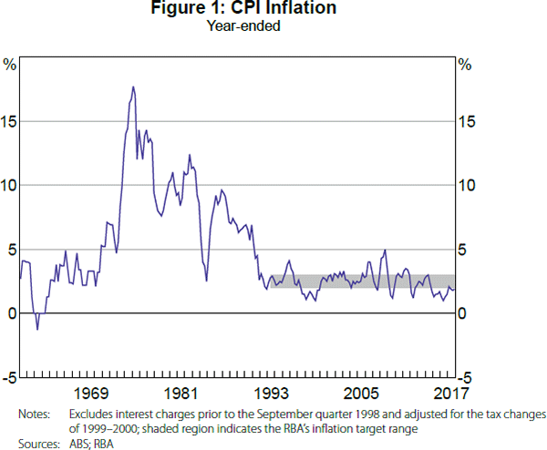
A quick look at the data in Figure 1 makes it clear that the introduction of inflation targeting corresponded to a stabilisation of the level of consumer price index (CPI) inflation in Australia around the numerical target range of 2–3 per cent introduced by the Reserve Bank of Australia (RBA) in 1993 (Stevens 1999). An important question is whether inflation targeting had other effects on the Australian economy, such as changing common movements in macroeconomic variables, including those related to the transmission of monetary policy shocks. Factor modelling provides a powerful and flexible way to investigate this empirical question in a data-rich environment.[1]
We compile a large panel of macroeconomic data for the Australian economy and conduct factor model analysis to investigate the effects of inflation targeting. Our analysis suggests that a sizeable portion of macroeconomic fluctuations for Australia can be captured by two common factors. This result is the same as was found for the US economy by Stock and Watson (2005) and many others. Standard selection criteria suggest the need for two to four common factors, with recursive estimates generally suggesting a possible decline in the number of common factors following the introduction of inflation targeting. This possible decline stands in contrast to findings for the US economy by Bai and Ng (2007) of a possible increase. A change in the number of factors is indicative of a change in the factor structure, with a decline implying a different type of structural change than an increase. We explore the particular nature of changes in the factor structure of the Australian economy in detail.
Based on the standard selection criteria, we estimate an approximate dynamic factor model of the Australian economy with three common factors. The estimation is based on quasi-maximum likelihood, as in Doz, Giannone and Reichlin (2011, 2012). Our estimates suggest that only two common factors explain a sizeable portion of macroeconomic fluctuations and they have clear ‘real’ and ‘nominal’ interpretations based on their factor loadings. We apply a recent test developed by Han and Inoue (2015) for a structural break in factor loadings and find a significant break, with the test statistics for two versions of the test maximised just before and after the introduction of inflation targeting in mid 1993 (Stevens 1999, 2003). Notably, both versions of the test would still be significant if the break were in 1993:Q1, corresponding to the introduction of inflation targeting in the next quarter, with 1993:Q1 close to the earliest date at which both test statistics are significant. Meanwhile, there is no evidence for additional structural breaks once accounting for the break at the estimated dates or in 1993:Q1.
Looking at the cross-sectional variation in the common and idiosyncratic components of macroeconomic variables before and after the introduction of inflation targeting, it is clear that there was a much larger reduction in the volatility of common components than idiosyncratic components. That is, inflation targeting has not just stabilised the level of inflation, but it also appears to have stabilised the common components of macroeconomic variables. This reduction in common volatility is broad based, applying to both real and nominal variables. Meanwhile, the fact that idiosyncratic components have remained relatively volatile suggests that signal-to-noise ratios for common and idiosyncratic movements in variables such as CPI inflation have declined, making the benefit of using factors rather than noisy individual variables even greater during the inflation-targeting era. Interestingly, recursive estimates of factor loadings for real gross domestic product (GDP) growth, CPI inflation, and the overnight cash rate (OCR) suggest a stabilisation rather than an abrupt change with the introduction of inflation targeting. This argues against a ‘Type 1’ break, in the terminology of Han and Inoue (2015), in which there is a change in cross-correlations related to common factors or, equivalently, an increase in the number of relevant factors. Instead, it is consistent with a change in the volatility of factors or, equivalently, a decrease in the number of relevant factors, consistent with our recursive estimates of the number of factors.
The results for the approximate dynamic factor model motivate us to consider a factor augmented vector autoregression (FAVAR) model in order to investigate possible changes in the transmission of monetary policy shocks following the introduction of inflation targeting. Even if cross-correlations of variables related to factors are relatively stable, shock identification will still be affected given changes in relative variances. For identification of monetary policy shocks, we follow Bernanke, Boivin and Eliasz (2005) and use estimated loadings to relate the full panel to a three-variable structural vector autoregressive (VAR) model that includes the ‘real’ and ‘nominal’ factors from our approximate dynamic factor model and the policy interest rate. Importantly, the two common factors are re-estimated from a subset of the panel that corresponds only to ‘slow-moving’ variables that should only respond with a lag to a monetary policy shock. We find that a contractionary monetary policy shock temporarily lowers real activity and inflation, with the ‘price puzzle’ almost completely resolved, as was found by Bernanke et al (2005) for the US data.[2] The CPI stabilises at a lower level, making it clear that the RBA targets inflation, not the price level (i.e. it lets ‘bygones be bygones’, as argued by Stevens (1999)). Structural break tests based on Qu and Perron (2007) suggest possible changes in VAR parameters around the introduction of inflation targeting and the global financial crisis (GFC). Sub-sample estimates suggest a resolution of the price puzzle and a flattening of the Phillips curve since the mid 2000s.
Our findings have important implications for monetary policy. First and foremost, they suggest that the benefits of inflation targeting are more than just in terms of stabilising the level of inflation, but also appear to involve reducing the common volatility of macroeconomic variables. This link in timing of a reduction in macroeconomic volatility with inflation targeting would be obscured somewhat by looking at real GDP growth on its own, but is clearer from the factor analysis. Relatedly, because idiosyncratic volatility has not reduced by as much as common volatility, our results suggest benefits to measuring real activity and price pressures using a factor modelling approach. The mitigation of a price puzzle for our FAVAR model provides an example of such a benefit. Despite apparent changes in the transmission of monetary policy, the factor modelling approach also allows for relatively precise estimation of the effects of a monetary policy shock in a data-rich environment and the possibility to relate the effects of policy to any variable in the panel, as well as any other variable that may only be available more recently due to data limitations, but for which we can estimate factor loadings. One clear implication of our FAVAR estimates is that the RBA currently pursues inflation targeting in line with its mandate, rather than price level targeting. Another clear implication is that, consistent with a flattening of the Phillips curve, the implied sacrifice ratio appears to have increased since the mid 2000s, suggesting caution against a shift to price level targeting.
The rest of this paper is organised as follows. Section 2 discusses the panel dataset, investigates the relevant number of common factors, presents estimates for an approximate dynamic factor model, and conducts break tests for the factor structure of the Australian economy. Section 3 examines the effects of inflation targeting on the factor structure of the Australian economy and draws some implications for monetary policy. Section 4 directly investigates possible changes in the transmission of monetary policy shocks by estimating a FAVAR model and also considers changes with the introduction of inflation targeting and during the inflation-targeting era, again drawing implications for monetary policy. Section 5 concludes. Full details of the dataset and estimation methods are provided in the appendices.
2. A Factor Model of the Australian Economy
2.1 An Australian macroeconomic panel dataset
We expand the panel datasets in Gillitzer, Kearns and Richards (2005) and Gillitzer and Kearns (2007) to cover 104 time series variables for the Australian economy from 1976:Q4 to 2017:Q2.[3] Due to data availability issues, the broader coverage of variables necessitates a later starting point for the sample than in Gillitzer et al (2005) and Gillitzer and Kearns (2007). However, the sample still includes 15 years before the introduction of inflation targeting in mid 1993 and nearly 25 years since its introduction.
Because many of the raw data series are non-stationary, we transform variables by taking logs and first differences as appropriate. As part of the transformation, we allow for a structural break in the mean levels of the price growth series in 1993:Q1, corresponding to the introduction of inflation targeting. This renders all of these series stationary without needing to take second differences. Once transformed to be stationary, we standardise all series by subtracting any remaining sample mean and dividing by the sample standard deviation. This implicitly gives each variable equal weight in the factor model.
In terms of broad categories, 42 per cent of the panel corresponds to real activity variables, 19 per cent to price variables, and 15 per cent to financial variables. Table 1 provides a more detailed breakdown into categories that we will refer to when looking at panel R2s for factors. Meanwhile, a list of all variables and their corresponding data transformations is provided in Appendix A.
| Category | Number |
|---|---|
| Expenditure | 20 |
| Income | 5 |
| Production | 19 |
| Employment | 8 |
| Surveys | 5 |
| Building & capital expenditure (capex) | 5 |
| Overseas transactions | 5 |
| Prices | 20 |
| Money & credit | 6 |
| Interest rates | 8 |
| Miscellaneous | 3 |
| Total | 104 |
|
Note: ‘Miscellaneous’ includes ‘Share price index’, ‘Real trade-weighted exchange rate index’, and the ‘Southern Oscillation Index’ Sources: ABS; RBA |
|
2.2 How many common factors?
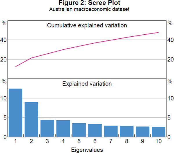
Figure 2 displays the ‘scree plot’ for the Australian macroeconomic panel dataset based on principle components analysis (PCA).[4] It provides a simple diagnostic for a likely number of relevant common factors. The largest two eigenvalues from PCA explain much more variation than all of the remaining eigenvalues. This is suggestive of two relevant common factors that capture about 13 per cent and 9 per cent of the joint variation in the macroeconomic variables, with the remaining ‘scree’ likely corresponding to much less important common factors or even idiosyncratic movements in some of the individual variables. This finding of two dominant common factors is consistent with findings for datasets for other countries, including for the US economy by Stock and Watson (2005).
Table 2 reports formal selection criteria results for the number of common factors. As can be seen from the cumulative explained variation in Figure 2, the next eight largest eigenvalues from PCA more than double the total variation explained. Thus, it is unclear whether two common factors are actually sufficient for the dataset. Starting with Bai and Ng (2002), formal selection criteria have been developed to determine the number of relevant common factors in a given dataset. The results in Table 2 capture this uncertainty about the number of common factors. While a majority of criteria select two common factors, there could be as many as seven relevant common factors.
| Number | |
|---|---|
| Bai and Ng (2002) | |
| PCP2 | 4 |
| lCP2 | 2 |
| Ahn and Horenstein (2013) | |
| Eigenvalue ratio (ER) | 2 |
| Growth ratio (GR) | 2 |
| Onatski (2010) | |
| Edge distribution (ED) | 7 |
|
Note: The upper bound on the maximum number of factors used with each method was 10 |
|
For our approximate factor model, we consider three common factors. We do so as a compromise between the 2–4 common factors suggested by the two Bai and Ng (2002) criteria. As will be seen with our estimates, two common factors appear to be sufficient to capture the main common variation in the dataset, but allowing for three common factors in the model makes this clear. Meanwhile, any evidence of more than three common factors, such as suggested by the Onatski (2010) criterion, could reflect changes in the factor structure, which we will also investigate in full detail.
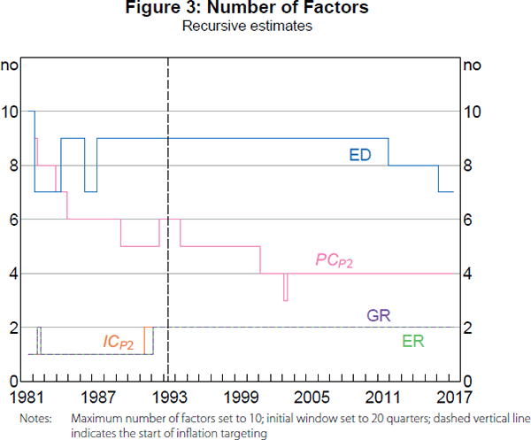
As a first step in looking at possible changes in the factor structure, Figure 3 reports recursive (expanding window) estimates of the number of common factors.[5] The end-of-sample estimates are the same as those reported in Table 2. What is notable, however, about the recursive estimates is that, among the criteria that suggest a larger number of common factors, there is a decline in the suggested number of factors since 1993:Q1. It is consistent with a particular type of structural change in which the factor structure simplifies over time due to an elimination of common variation and, thus, corresponds to a reduction in volatility rather than a change in cross-correlations explained by common factors. Notably, this decline contrasts with findings by Bai and Ng (2007) for the US economy of an increase in the suggested number of factors in recent years. Again, we will investigate this possibility in full detail.
2.3 Estimates for an approximate dynamic factor model
Based on the Bai and Ng (2002) selection criteria, we estimate an approximate dynamic factor model with three common factors:
where Yt is the data, Λ are the factor loadings,
Ft are the factors and εt is the
idiosyncratic component. Yt and εt are
N × 1, Λ is N × 3, Ft and ηt
are 3 × 1. The factors are assumed to follow a VAR(1), Ft = Φ(L)Ft
− 1 + ηt, while Φ(L) is a 3 × 3
conformable lag polynomial. An approximate dynamic factor model allows the elements of
εt to be weakly dependent across series and time, but they are
uncorrelated with the common factors,  .[6]
.[6]
We conduct initial ‘static’ estimation using PCA, following Stock and Watson (2005).[7] Then, using these static estimates, we calculate dynamic factor estimates using quasi-maximum likelihood estimation (QMLE) for a VAR of the factors with one lag based on Schwarz information criterion (SIC) and Kalman filter/smoother recursions via the expectation maximisation (EM) algorithm, following Doz et al (2011, 2012). See Appendix B for more details.
Figure 4 displays the static and dynamic estimates of the three common factors.[8] There is a strong coherence between the estimates for the first two factors, which display considerable persistence. There is less evidence of a link between the estimates of the third factor, which also appears to be far less persistent. An explanation could be that the static estimates of the third factor capture some lagged dynamics of the first two factors, but it is mostly noise when considering dynamic factor estimation with a VAR(1) structure. Meanwhile, the dynamic estimates of the third factor turn out to explain very little variation of the panel dataset.
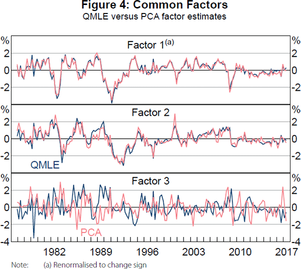
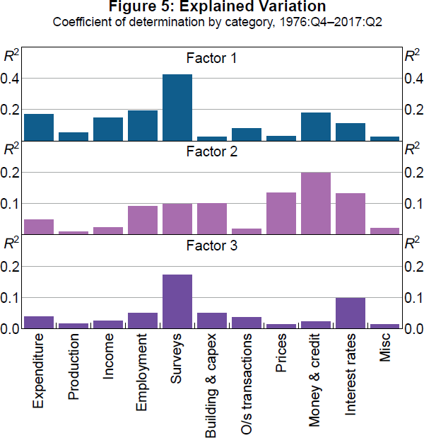
Figure 5 reports the variation of data in different categories explained by the common dynamic factors based on panel R2s that capture the fraction of the variance of a series explained by a given common factor. The fact that these are all reasonably low suggests that variables in each category are subject to considerable idiosyncratic variation. It is also clear based on the categories that the first factor corresponds more to ‘real’ variables such as measures of expenditure, employment, and activity surveys, while the second factor corresponds more to ‘nominal’ variables, such as prices, money, credit, and interest rates. Notably, we find that interest rate spreads in particular load on both factors, which likely reflects their information content about both real activity and inflation. As mentioned above, the third factor explains very little variation of the panel, with the highest R2s corresponding to activity surveys and interest rates. Thus, it may capture something about expectations of future real activity or ‘sentiment’, but it is possibly just noise that can be dropped from the model.
2.4 Breaks in the factor structure?
As noted above, one reason why some selection criteria might suggest more than two factors could be due to changes in the factor structure. We formally test for structural breaks using an approach recently proposed by Han and Inoue (2015).[9] The null hypothesis of their test is that all factor loadings are constant over time against the alternative that a non-negligible fraction of factor loadings have changed. The test makes use of the fact that the presence of a structural break in factor loadings implies changes in the second moments of the factors. Han and Inoue (2015) note that a change in the volatility of factors or in factor loadings would not be separately identified, so a rejection could reflect either or both. The idea of a change in dynamic factor loadings in the sense of being equivalent to additional factors in a PCA setting corresponds to a ‘Type 1’ break, where the change in the factor structure reflects a change in cross-correlations between variables related to common factors. By contrast, the idea of a change in the volatility of factors corresponds to a ‘Type 2’ break, where the change in the factor structure reflects a change in the volatility of variables related to common factors, but with the same cross-correlations between variables related to common factors. Our earlier finding of a reduction in the number of factors implied by some of the criteria in Figure 3 is more consistent with a Type 2 break than a Type 1 break, but we will examine issue this directly.
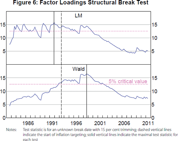
Figure 6 plots the Han and Inoue (2015), LM and Wald test statistics for a structural break in factor loadings. In both cases, we can reject the null of no break, with the LM test statistic maximised in 1991:Q4 and the Wald test statistic maximised in 1998:Q3. Notably, however, both test statistics are still significant if the break occurred in 1993:Q1 with the introduction of inflation targeting, which is close to the earliest date at which both test statistics are significant. Thus, the results for Han and Inoue's (2015) test are consistent with the idea that the introduction of inflation targeting led to a change in the factor structure of the Australian economy. Furthermore, we note that the there is no support for an additional break, whether the first break is set to have occurred at the estimated dates or in 1993:Q1. Given a break in the factor structure around the time of the introduction of inflation targeting, we turn next to an investigation of what effects it had on the Australian economy.
3. Effects of Inflation Targeting
3.1 Decline in common shocks
We find that the introduction of inflation targeting corresponded to a much larger reduction in the volatility of common components of macroeconomic time series than idiosyncratic components. To see this, we calculate the cross-sectional variance of common components, which reflects the variability of common factors, and of idiosyncratic components, which reflects the residual variability of the data, at each point in time. Figure 7 plots measures of common and idiosyncratic volatility over the whole sample for: (i) all of the variables, (ii) just real variables, (iii) just nominal variables, and (iv) just price variables. The pattern is consistent in all of the cases. Although there are still peaks in the volatility measures after 1993 that seem to be related to events such as the introduction of the goods and services tax in 2000 (idiosyncratic volatility) and the GFC in 2007–09 (both common and idiosyncratic volatility), there is clearly lower average common volatility since the introduction of inflation targeting. The absence of a recession in Australia since 1993 could help explain the relative lack of peaks in common volatility that occurred with the recessions in the early 1980s and 1990s. However, the common volatility is still generally lower after the introduction of inflation targeting than it was even during expansions prior to inflation targeting. Furthermore, contrary to recessions being the primary driver of volatility, the idiosyncratic volatility looks only slightly lower on average since 1993, and this is not even clear for the price variables. Meanwhile, because the reduction of idiosyncratic volatility is not as large as the reduction of common volatility, signal-to-noise ratios for individual variables that proxy for the common factors have clearly dropped since the introduction of inflation targeting.
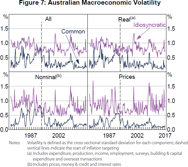
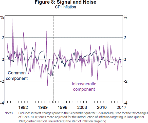
Figure 8 illustrates the decline in the signal-to-noise ratio by plotting the common and idiosyncratic components of (adjusted and standardised) CPI inflation. The variation in both components seems to have lessened somewhat, but much more so for the common component. Thus, a higher proportion of the quarterly fluctuations in CPI inflation reflect noise since the introduction of inflation targeting. A direct implication for monetary policy is that it makes sense to ‘look through’ some of the high frequency movements in CPI inflation. Such movements are more likely to be reflecting noise rather than a persistent change in underlying inflationary pressures. Furthermore, the dynamic factor model provides a way to extract a signal about underlying inflationary pressures from a noisy series such as CPI inflation.
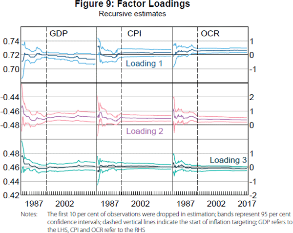
3.2 Stabilised factor loadings
To further investigate the nature of the change in the factor structure, we calculate recursive estimates of factor loadings for real GDP growth, CPI inflation and the OCR on the estimated factors.[10] Figure 9 plots these recursive estimates along with 95 per cent confidence bands.[11] Real GDP growth loads significantly on all three factors, CPI inflation only loads significantly on the second factor, and the OCR loads significantly on the first two factors. The estimated loadings for all three variables on the first factor are positive (although, again, insignificant for CPI inflation). This suggests that the first factor could reflect demand pressures in the economy. The estimated loadings for the second factor are negative on real GDP growth and positive for CPI inflation and the OCR, suggesting the factor could reflect supply-side inflationary pressures. The estimated loadings for the third factor are positive for real GDP growth and effectively zero for CPI inflation and the OCR, suggesting that factor could reflect high frequency real activity movements that do not spill over into inflation or affect monetary policy. Meanwhile, it is quite notable that the recursive estimates of the factor loadings seem to stabilise rather than jump with the introduction of inflation targeting. This is consistent with a Type 2 break.
3.3 Interpretation and implications
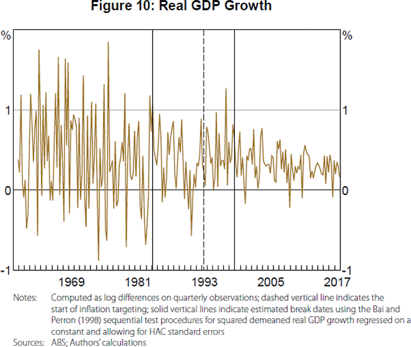
The structural break analysis suggests that inflation targeting has done more than just stabilise the level of inflation in Australia. It has also reduced the volatility of common movements in macroeconomic variables and possibly reduced the number of common factors in the economy. This reduction in volatility is not just in price growth and other nominal variables but is broad based. One possibility is that it could be driven by an elimination of ‘sunspot’ shocks following the introduction of inflation targeting due to its provision of a clear nominal anchor for inflation expectations.[12] Notably, the estimated timing of the reduction in macroeconomic volatility that is linked to the introduction of inflation targeting is different than that implied by looking at real GDP growth on its own (Figure 10).[13] This suggests that there is a clear benefit from using factor analysis in this case. The timing is also different than that of the volatility reduction in US output growth and inflation (the mid 1980s) found in numerous studies (e.g. Stock and Watson 2003), which suggests it is not due to any changes in global factors at the same time as the introduction of inflation targeting in Australia.
In addition, the larger drop in the volatility of common components relative to idiosyncratic components implies an increased benefit of looking at common factors to eliminate noise in individual observed variables. Notably, price measures, including CPI inflation, have particularly large idiosyncratic components, while our factor model estimates suggest that the RBA can ‘look through’ most quarterly fluctuations in these measures and focus on underlying measures such as the common component of price growth variables provided by our approximate dynamic factor model.
The stability of the factor loadings is reassuring for the use of a factor model to capture real and nominal fluctuations in the Australian economy. However, even with stable loadings, changes in relative variances of shocks in the economy can result in changes in the dynamic interactions of variables. For example, the transmission of monetary policy shocks may have changed with the introduction of inflation targeting. We turn to this issue next.
4. Transmission of Monetary Policy
Based on the apparent factor structure of the Australian economy, we develop a FAVAR model to examine the transmission of monetary policy shocks, including possible changes due to the introduction of inflation targeting.
4.1 FAVAR model
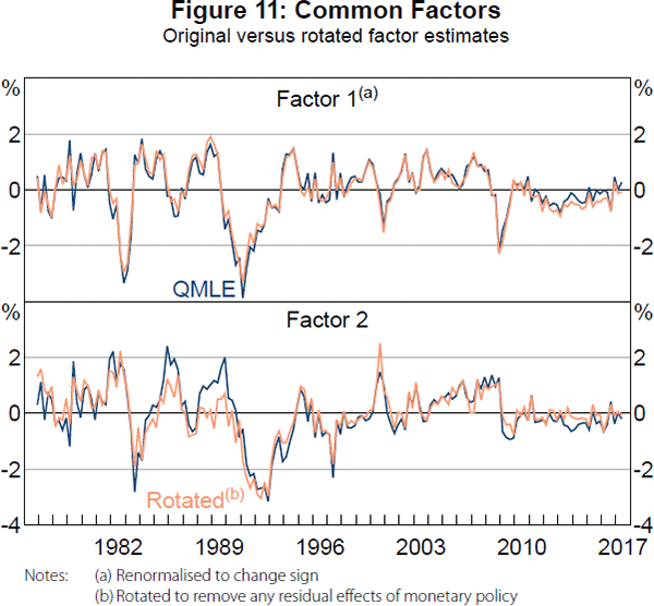
Following Bernanke et al (2005), we estimate a FAVAR model based on their preferred specification of using the policy interest rate as an observed factor. The model uses factor loadings to relate the full panel of data to a three-variable VAR that includes the first two common factors corresponding to real and nominal fluctuations and the OCR. We extract the first two factors from a subset of the panel that corresponds only to ‘slow-moving’ variables. It excludes, for example, survey measures, oil prices, commodity prices, financial variables and the exchange rate. The full list is given in Table A1. Crucially, the panel excludes the OCR and the factors are rotated to remove any residual effects of the policy rate. Despite these changes, the extracted factors are very similar to the original factors estimated from the full panel (Figure 11). Then, monetary policy shocks are identified by assuming they are contemporaneously uncorrelated with other shocks that drive the factors.[14] See Appendix C for full details.
4.2 Full sample estimates
Before considering structural change, we start by estimating a FAVAR with two lags (based on the SIC) for the full sample of 1976:Q4–2017:Q2 to provide benchmark results. Given FAVAR parameter estimates, we calculate impulse response functions (IRFs) for a surprise 25 basis point increase in the OCR, with reported 95 per cent confidence bands based on 500 bootstrap replications.
Figure 12 plots IRFs for the OCR and the two factors. The OCR increases 25 basis points on impact, by construction, and then it gradually reverts back to its initial level, while both factors contract significantly at business cycle horizons. Given the loadings for these factors (positive for real GDP growth on the first factor and positive for CPI inflation on the second factor), these results are consistent with the interpretation of the identified monetary policy shock as being contractionary.
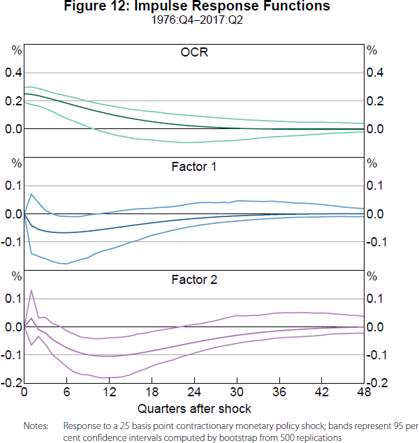
Figure 13 directly examines the implied IRFs for real GDP growth and CPI inflation. The point estimates still show contractionary effects, although the response of real GDP growth is no longer significant, reflecting the fact that real GDP growth also loads negatively on the second factor in addition to loading positively on the first factor. The response of CPI inflation is very similar to the response of the second factor, reflecting an insignificant loading of CPI inflation on the first factor. Accumulated responses are also reported to show the implied effects of a monetary policy shock on the log levels of real GDP and the CPI. Consistent with long-run monetary neutrality, there is no significant long-run effect on log real GDP. Meanwhile, log CPI is permanently lower following the contractionary monetary policy shock. This reflects the dynamics of the OCR in response to the policy shock, with the RBA gradually returning the policy rate back to its original level, but not overshooting in order to reverse the initial effects of the shock on the price level. That is, the IRFs are consistent with the RBA targeting the inflation rate, not the price level, and letting ‘bygones be bygones’.
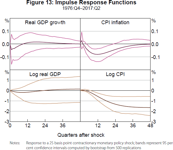
The point estimate for the response of CPI inflation to a contractionary monetary policy shock is slightly positive at the one quarter horizon. However, it is insignificant and the point estimates are negative and often significantly so at subsequent horizons. Thus, these IRFs largely resolve the so-called ‘price puzzle’, as Bernanke et al (2005) did with their FAVAR for the US economy.[15] The price puzzle has been particularly challenging to solve for Australian SVARs, as discussed in Bishop and Tulip (2017). So our result is particularly encouraging for using a FAVAR to estimate the effects of monetary policy shocks on the Australian economy.
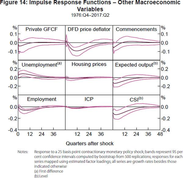
A benefit of the FAVAR model is that it allows us to examine the effects of a monetary policy shock on any variable in the panel (and even variables not in the panel, as long as we can determine relevant loadings on the factors). Figure 14 plots the IRFs for a selection of other variables that reflect different aspects of the Australian economy. The variables are private gross fixed capital formation (GFCF), the domestic final demand (DFD) price deflator, housing commencements, the unemployment rate, housing prices, a survey of expected output, total employment growth, an index of commodity prices (ICP), and a consumer sentiment index (CSI). The series are transformed to be stationary where appropriate and as noted in the figure. The IRFs behave as expected given a contractionary monetary policy shock. For example, DFD price deflator inflation behaves very similarly to CPI inflation, the unemployment rate increases significantly at business cycle horizons, and consumer sentiment falls significantly at business cycle horizons.
4.3 Breaks in the FAVAR?
Given the benchmark full sample results, we now consider whether the introduction of inflation targeting changed the FAVAR parameters or whether they changed at any other point of the sample. To test for structural breaks in the FAVAR, we apply the Qu and Perron (2007) procedures. In principle, the methods in Qu and Perron can be applied to a linear system of regression equations with multiple structural breaks in mean or variance. However, given the large number of parameters for the FAVAR model, we need to apply tests for structural breaks equation by equation. Tables 3 and 4 report the results of Qu and Perron's (2007) supLR tests and sequential tests for each equation of the VAR portion of the model allowing for breaks in conditional mean and variance. Given a VAR set-up, we assume no residual serial correlation. We consider a maximum of three breaks with 15 per cent trimming from sample end points and between breaks.
The results support the existence of structural change in all three dynamic equations of the FAVAR, with the sequential tests providing some insight into the number and timing of the breaks. For the first factor, there appear to be two breaks, estimated to have occurred in 1990:Q1 and 2010:Q2. For the second factor, there appears to have been one break in 2011:Q1. For the OCR, there appear to be two breaks, estimated to have occurred in 1990:Q3 and 2011:Q1.
| Number | Test statistic | Critical value (5 per cent) |
||
|---|---|---|---|---|
| Factor 1 | Factor 2 | OCR | ||
| 1 | 43.31 | 45.77 | 197.80 | 24.21 |
| 2 | 78.91 | 69.89 | 268.87 | 40.09 |
| 3 | 99.33 | 91.23 | 290.40 | 55.00 |
| Notes: Test is for a break in the conditional mean and variance; number of breaks tested for is three; trimming parameter is set to 0.15; total number of parameters in each equation is eight | ||||
| Seq(ℓ + 1|ℓ) | Factor 1 | Factor 2 | OCR | Critical value (5 per cent) | |||||
|---|---|---|---|---|---|---|---|---|---|
| Test statistic | H0 date | Test statistic | H0 date | Test statistic | H0 date | ||||
| Seq(2|1) | 35.60 | 1990:Q1 | 24.12 | 2011:Q1 | 71.07 | 1990:Q3 | 26.58 | ||
| Seq(3|2) | 22.93 | 2010:Q2 | na | na | 26.49 | 2011:Q1 | 27.58 | ||
|
Notes: Test is for a break in the conditional mean and variance; number of breaks tested for is three; trimming parameter is set to 0.15; total number of parameters in each equation is eight |
|||||||||
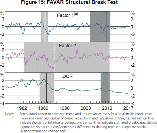
Figure 15 reports 95 per cent confidence sets for the structural break dates.[16] The confidence sets vary considerably in their precision for the different variables. However, the results broadly suggest that we should account for two breaks in the FAVAR, with the first break around the introduction of inflation targeting and the second break around the GFC. Technically, the apparent timing of the first break for the first factor and the OCR based on the 95 per cent confidence sets occurred just after the introduction of inflation targeting (the data are not informative at all about the timing of a break for the second factor). However, for simplicity of interpretation and because it can be shown that 1993:Q1 is within the 99 per cent confidence sets, we consider our first sub-sample for the FAVAR to be up to the introduction of inflation targeting, although our FAVAR estimates would be similar if we used either of the earlier estimated break dates in 1990. For the second break, we find the FAVAR estimates are highly imprecise using only data after the GFC, which is likely due to few surprise changes in the OCR during this period. If we extend the sub-sample back to begin in the mid 2000s, which is consistent with 95 per cent confidence sets for the two factors and what can be shown to be the 99 per cent confidence set for the OCR, the FAVAR estimates are relatively more precise. Thus, we consider the last sub-sample for our FAVAR to begin in 2005:Q1, which is consistent with the earliest second break for the first factor in the 95 per cent confidence set. The results would be similar, but increasingly less precise, if we moved the start of the last sub-sample to later in the 2000s.
4.4 Sub-sample estimates
Based on the structural break test results, we split the sample into three regimes: pre-inflation targeting, 1976:Q4–1993:Q1; early inflation targeting, 1993:Q2–2004:Q4; and late inflation targeting, 2005:Q1–2017:Q2. The apparent changes in the VAR parameters motivate our consideration of this sub-sample analysis. In particular, a change in any of the reduced-form slope coefficients or cross-correlations for the forecast errors should lead to different identified structural shocks for the FAVAR and, therefore, different estimated IRFs.
Looking at the top row of Figure 16, the dynamics of the OCR following a contractionary shock have changed considerably over the full sample of 1976:Q4–2017:Q2. In the pre-inflation-targeting period, the RBA appeared to quickly bring the OCR back to its previous level and even significantly lowered it for a while afterwards. In the early inflation-targeting period, the RBA appears to have introduced a bit more persistence into the OCR and seems to have deliberately avoided any expansionary overshooting following a contractionary shock. In the late inflation-targeting period, the RBA further increased the persistence of the OCR, but may have allowed some expansionary offset at long horizons, although it is not significant.
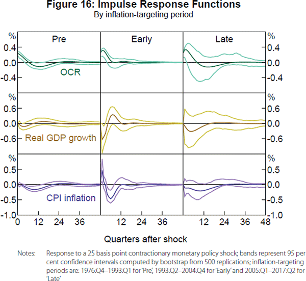
In terms of the effects of a contractionary monetary policy, the second and third rows of Figure 16 display the sub-sample responses of real GDP growth and CPI inflation, respectively. In the pre-inflation-targeting period, the contractionary shock always decreases real GDP growth at short horizons, but the lower OCR at longer horizons seems to have stimulatory effects. In the early inflation-targeting period, the estimated response of real GDP is quite volatile, perhaps reflecting a less successful identification of a policy shock for this sub-sample, as evidenced by a return of a price puzzle in the response of CPI inflation. The strong estimated rebound of real GDP growth could then reflect too quick of a decrease in the policy rate back to zero in the face of an underlying inflationary shock that leads to a policy contraction.[17] In the late inflation-targeting period with the policy framework well established, the more persistent contraction of monetary policy has stronger effects on real GDP growth and CPI inflation, without a price puzzle.
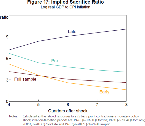
Using the estimated impulse responses for a monetary policy shock, we examine implied sacrifice ratios for the Australian economy by calculating the accumulated response of real GDP relative to the response of CPI inflation. Figure 17 plots these ratios at the one- to two-year horizon for the different sub-samples, with the full sample as a benchmark. It appears that the sacrifice ratio initially fell with the introduction of inflation targeting, consistent with the idea that a credible nominal anchor can allow inflation expectations to adjust more quickly. However, the sacrifice ratio rose considerably after the mid 2000s, perhaps corresponding to a flattening of the Phillips curve similar to Gillitzer and Simon (2015). Of course, if this flattening is due to an anchoring of inflation expectations, then a high sacrifice ratio is not a problem in and of itself as the RBA should not need to undertake a large disinflation in the first place, although it provides a caution against the RBA adopting a price level target that could require larger disinflations following a temporary increase in measured inflation.
5. Conclusion
Factor model analysis provides a useful way to investigate the effects of inflation targeting and the transmission of monetary policy shocks for the Australian economy. Notably, inflation targeting has not just stabilised the level of inflation, but it has also reduced the volatility of common movements in macroeconomic variables. A drop in the implied signal-to-noise ratios for macroeconomic data given a larger decline in common volatility relative to idiosyncratic volatilities implies an increased benefit of considering common factors instead of focusing only on individual noisy series such as CPI inflation. Our FAVAR estimates suggest that monetary policy shocks have become more persistent and their effects amplified, while sacrifice ratios and the implied slope of the Phillips curve have also changed over time.
The flexibility of factor modelling allows us to propose a number of possible extensions to our analysis. We plan to consider alternative models of structural change in the future, such as: a Markov-switching dynamic factor model used by Diebold and Rudebusch (1996), Chauvet (1998), Kim and Nelson (1998) and Camacho, Perez-Quiros and Poncela (2015); or a time-varying parameter dynamic factor model used in Korobilis (2013). These alternative models will allow us to determine if there is any recurring dependence in the effects of monetary policy shocks or other identified shocks (e.g. foreign shocks) on the state of the business cycle, or if there are other slower moving changes. We also plan to utilise methods recently developed by Koopman, Mesters and Schwaab (2018) for jointly estimating level and volatility factors and their interaction. This will allow us to examine the role of uncertainty in driving the Australian economic conditions in a data-rich environment. Also, we plan to consider more observed factors, such as commodity prices, US real GDP growth, US CPI inflation, the federal funds rate and government spending, in the FAVAR in order to consider the dynamic effects of different types of structural shocks and to possibly better identify monetary policy shocks.
Appendix A: Australian Macroeconomic Dataset
| Variable | Category | Transformation | Slow variable |
|---|---|---|---|
| Gross domestic product (GDP) | Expenditure | Δlog(xt) | Yes |
| Non-farm GDP | Expenditure | Δlog(xt) | Yes |
| GDP per capita | Expenditure | Δlog(xt) | Yes |
| Public final demand | Expenditure | Δlog(xt) | Yes |
| Private final demand | Expenditure | Δlog(xt) | Yes |
| Private gross fixed capital formation (GFCF) | Expenditure | Δlog(xt) | Yes |
| Household consumption (HC) | Expenditure | Δlog(xt) | Yes |
| HC: Cigarettes and tobacco | Expenditure | Δlog(xt) | Yes |
| HC: Alcoholic beverages | Expenditure | Δlog(xt) | Yes |
| HC: Clothing and footwear | Expenditure | Δlog(xt) | Yes |
| HC: Food | Expenditure | Δlog(xt) | Yes |
| HC: Household equipment | Expenditure | Δlog(xt) | Yes |
| HC: Purchase of vehicles | Expenditure | Δlog(xt) | Yes |
| HC: Rent and other dwelling services | Expenditure | Δlog(xt) | Yes |
| HC: Hotels, cafes and restaurants | Expenditure | Δlog(xt) | Yes |
| HC: Transport services | Expenditure | Δlog(xt) | Yes |
| Private GFCF: Dwellings: Alterations and additions | Expenditure | Δlog(xt) | Yes |
| Private GFCF: Dwellings: New and used | Expenditure | Δlog(xt) | Yes |
| Private non-farm inventories to total sales | Expenditure | Δxt | Yes |
| Changes in inventories | Expenditure | xt | Yes |
| Gross domestic income | Income | Δlog(xt) | Yes |
| Gross operating surplus: Financial corporations | Income | Δlog(xt) | Yes |
| Gross operating surplus: Private non-financial | Income | Δlog(xt) | Yes |
| Gross operating surplus: Public non-financial | Income | Δlog(xt) | Yes |
| Household disposable income | Income | Δlog(xt) | Yes |
| Agriculture, forestry and fishing | Production | Δlog(xt) | Yes |
| Mining and exploration | Production | Δlog(xt) | Yes |
| Manufacturing | Production | Δlog(xt) | Yes |
| Electricity, gas and water services | Production | Δlog(xt) | Yes |
| Construction | Production | Δlog(xt) | Yes |
| Wholesale trade | Production | Δlog(xt) | Yes |
| Retail trade | Production | Δlog(xt) | Yes |
| Accommodation and food services | Production | Δlog(xt) | Yes |
| Transportation | Production | Δlog(xt) | Yes |
| Information media and telecommunications | Production | Δlog(xt) | Yes |
| Financial and insurance services | Production | Δlog(xt) | Yes |
| Rental hiring and real estate services | Production | Δlog(xt) | Yes |
| Professional, scientific and technical services | Production | Δlog(xt) | Yes |
| Administration and support services | Production | Δlog(xt) | Yes |
| Public administration and safety | Production | Δlog(xt) | Yes |
| Education and training | Production | Δlog(xt) | Yes |
| Healthcare and social assistance | Production | Δlog(xt) | Yes |
| Arts and recreation services | Production | Δlog(xt) | Yes |
| Other services | Production | Δlog(xt) | Yes |
| Full-time employment | Employment | Δlog(xt) | Yes |
| Part-time employment | Employment | Δlog(xt) | Yes |
| Total employment | Employment | Δlog(xt) | Yes |
| Unemployment rate | Employment | Δxt | Yes |
| Labour productivity | Employment | Δlog(xt) | Yes |
| Real unit labour costs | Employment | Δlog(xt) | Yes |
| Average weekly earnings | Employment | Δlog(xt) | Yes |
| Average weekly hours worked | Employment | Δlog(xt) | Yes |
| Capacity utilisation (net balance) | Surveys | xt | No |
| General business situation (next 6 months net balance) | Surveys | xt | No |
| Output actual (change in past 3 months net balance) | Surveys | xt | No |
| Output expected (change in next 3 months net balance) | Surveys | xt | No |
| Consumer sentiment index | Surveys | xt | No |
| Commencements: Total new houses and flats excl conversion | Building & capex | Δlog(xt) | No |
| Completed: Total new houses and flats excl conversion | Building & capex | Δlog(xt) | Yes |
| Approvals: Private new houses and flats | Building & capex | Δlog(xt) | No |
| Approvals: Government new houses and flats | Building & capex | Δlog(xt) | No |
| Approvals: Total new houses and flats | Building & capex | Δlog(xt) | No |
| Current account (per cent of GDP) | Overseas transactions | Δxt | Yes |
| Services imports | Overseas transactions | Δlog(xt) | Yes |
| Services exports | Overseas transactions | Δlog(xt) | Yes |
| Goods debits | Overseas transactions | Δlog(xt) | Yes |
| Goods credits | Overseas transactions | Δlog(xt) | Yes |
| Consumer price index (CPI): All groups | Prices | Δlog(xt) | Yes |
| CPI: Food and non-alcoholic beverages | Prices | Δlog(xt) | Yes |
| CPI: Alcohol and tobacco | Prices | Δlog(xt) | Yes |
| CPI: Clothing and footwear | Prices | Δlog(xt) | Yes |
| CPI: Housing | Prices | Δlog(xt) | Yes |
| CPI: Household equipment and services | Prices | Δlog(xt) | Yes |
| CPI: Transportation | Prices | Δlog(xt) | Yes |
| CPI: Communication | Prices | Δlog(xt) | Yes |
| CPI: Goods component | Prices | Δlog(xt) | Yes |
| CPI: Services component | Prices | Δlog(xt) | Yes |
| Established house prices | Prices | Δlog(xt) | Yes |
| Oil prices | Prices | Δlog(xt) | No |
| GDP price deflator | Prices | Δlog(xt) | Yes |
| Household final consumption expenditure price deflator | Prices | Δlog(xt) | Yes |
| Private GFCF price deflator | Prices | Δlog(xt) | Yes |
| Domestic final demand (DFD) price deflator | Prices | Δlog(xt) | Yes |
| Export price index: Goods and services credits | Prices | Δlog(xt) | Yes |
| Import price index: Goods and services debits | Prices | Δlog(xt) | Yes |
| Terms of trade | Prices | Δlog(xt) | Yes |
| Index of commodity prices (ICP) | Prices | Δlog(xt) | No |
| Money: M1 | Money & credit | Δlog(xt) | No |
| Money: M3 | Money & credit | Δlog(xt) | No |
| Money: Broad money | Money & credit | Δlog(xt) | No |
| Credit: Total | Money & credit | Δlog(xt) | No |
| Credit: Other personal | Money & credit | Δlog(xt) | No |
| Credit: Business | Money & credit | Δlog(xt) | No |
| Overnight cash rate (OCR) | Interest rates | Δxt | No |
| Real OCR | Interest rates | Δxt | No |
| 3-month bank bill | Interest rates | Δxt | No |
| 5-year Australian Government security (AGS) | Interest rates | Δxt | No |
| 10-year AGS | Interest rates | Δxt | No |
| 3-month bank bill spread to OCR | Interest rates | xt | No |
| 5-year AGS spread to OCR | Interest rates | xt | No |
| 10-year AGS spread to OCR | Interest rates | xt | No |
| Share price index | Miscellaneous | Δlog(xt) | No |
| Real trade-weighted exchange rate index (TWI) | Miscellaneous | Δlog(xt) | No |
| Southern Oscillation Index (SOI) | Miscellaneous | xt | No |
|
Notes: Seasonally adjusted data are used when available; monthly series are converted to quarterly by taking the three-month average; ‘Slow variable’ refers to whether the respective series is used to extract ‘slow-moving’ factors as part of the procedure when estimating the FAVAR model; the ‘Money & credit’ series are break adjusted Sources: ABS; Bureau of Meteorology; RBA |
|||
Appendix B: Quasi-maximum Likelihood Estimation
Following Doz et al (2012), we consider an approximate dynamic factor model estimated by QMLE. The estimation is ‘quasi’ in the sense that the underlying model is misspecified. The source of misspecification relates to omitted cross-sectional correlation of the idiosyncratic components. Doz et al (2012) show that the effects of misspecification on the estimation of the common factors is negligible for large sample size T and cross-section dimension N. The state-space form of the QMLE dynamic factor model is given as follows:
The parameter matrices of the measurement and state equations have the following structure:
where lr is an r-dimensional identity matrix and 0r is an r-dimensional matrix of zeros. The covariance matrix of εt in the measurement equation is given by R with dimension N × N and is restricted to be a diagonal matrix. In the state equation, the covariance matrix of ηt corresponds to the r × r matrix Q while G is a rp × r selector matrix. In our work we set p = 1 based on the SIC which leads to Equation (1).
The QML estimator is implemented using the Kalman filter/smoother and the EM algorithm. To do this, we initialise the Kalman filter/smoother recursions using the first r PCA-based estimates of the factors and OLS estimates of the parameters Λ,Φ(L),R, and Q, treating the PC factors as the true common factors. This represents the ‘expectation’ step and provides a new estimate of the common factors given the estimated parameters. Based on the updated estimate of the factors, we compute new parameter estimates via OLS, which is the ‘maximisation’ step. These two steps are repeated until the algorithm converges. We judge convergence to be when cm is less than 10−6 with cm given by:
where θ is a vector of the model parameters and m = 1,…,M
is the number of evaluations needed to achieve convergence up to a maximum
M set by the researcher. We set M = 1,000 but the number of
evaluations needed in all cases we considered was much less than 100.  is the log-likelihood function given as:
with the initial state F0 = 0rp and initial
state variance  . See Ghahramani and Hinton (1996) for
more details.
. See Ghahramani and Hinton (1996) for
more details.
A convenient feature of this specification is that the computational complexity of the Kalman filter/smoother depends only on the number of states, which in our case corresponds to the number of factors r, and is independent of the size of the cross-section N.
Note, while the EM algorithm will converge, it is not guaranteed to find the global maximum and can converge to a local maximum. However, the chance of this occurring can be offset by starting the algorithm, as we do, with the PCA estimates which are consistent for large cross-sections.
The main reason we use this estimation method relates to its potential to improve efficiency of the estimates of the common factors. This comes from explicitly accounting for factor dynamics. Doz et al (2012) show the efficiency improvements are relevant when there are more common factors to estimate. Other desirable features of this method (which we do not explore in our work) relate to structural analysis by allowing the researcher to impose restrictions on the factor loadings to extract shocks. Furthermore, the method is capable of handling either missing or mixed frequency data.
Appendix C: FAVAR Estimation
Here we describe the FAVAR model estimation in detail. Let Rt be the official cash rate. Suppose that additional economic information can be summarised by a k × 1 vector of unobserved factors Ft, where k is small and is not necessarily equal to r as determined via some formal selection criteria. We can think of the unobserved factors as possibly capturing variation in economic activity or price pressures that may not be readily proxied by any particular individual observed variable, but are important in a wide range of economic data series. Assume the joint dynamics of Ft, and Rt are given by the following equation:
where Φ(L) is a conformable lag polynomial of finite order p. We set p = 2 in our case based on SIC. We then assume that what Bernanke et al (2005) call ‘informational’ time series Yt are related to the unobserved factors Ft and observed Rt by the equation:
where ΛF is an N × k matrix of common factor loadings, ΛR is an N × 1 vector of Rt loadings and et is an N × 1 vector of error terms with mean zero that are assumed to display a small amount of cross-correlation.
We consider only one approach to estimating the FAVAR (Bernanke et
al (2005) consider two, one via PCA and the other via Bayesian estimation). We
use their two-step method based on the PCA estimator, but we replace this with the
QML estimates of the factors. This is not new as Bernanke and Boivin (2003) did
something similar using a mixed frequency panel for the US economy. Denote the
estimated common factors of Yt by  .
Because corresponds to an arbitrary linear combination
of its arguments, obtaining
.
Because corresponds to an arbitrary linear combination
of its arguments, obtaining  involves determining the
part of that is not spanned by Rt.
involves determining the
part of that is not spanned by Rt.
Because Rt is not explicitly imposed as a common component in
the first estimation step, any of the linear combinations underlying could involve Rt. Bernanke et al (2005) argue that it would not be valid to simply estimate
a VAR based on and identify the policy shock
recursively. Instead, they argue that the direct dependence of the common factors of
Yt on Rt must be removed first.
If linear combinations implicit in were known, this
would involve subtracting Rt times the associated coefficient
from each of the elements of . However, because they are
unknown, Bernanke et al propose to estimate the coefficients
through a multiple regression of the form:
where  is an estimate of all the common components other
than Rt. Bernanke et al (2005) suggest one
way to obtain is to extract factors from a subset of
slow-moving variables, which by assumption are not affected contemporaneously by
Rt. Then is constructed as
is an estimate of all the common components other
than Rt. Bernanke et al (2005) suggest one
way to obtain is to extract factors from a subset of
slow-moving variables, which by assumption are not affected contemporaneously by
Rt. Then is constructed as  and a VAR in and Rt
is estimated using ordinary least squares and identified recursively.
and a VAR in and Rt
is estimated using ordinary least squares and identified recursively.
Note that the key assumption is that most of the forecast error for Rt reflects monetary policy shocks, not an endogenous response to economic conditions. Finally, because this second step involves the presence of generated regressors, we use the bootstrap and 500 replications to compute confidence bands for the impulse response functions displayed in Section 4.
Footnotes
Luke Hartigan is from the Economic Research Department of the Reserve Bank of Australia (RBA) and James Morley is from the University of Sydney. The views expressed in this paper are those of the authors and not necessarily those of the RBA. [*]
See Stock and Watson's (2016) survey of factor modelling and its use in examining the effects of structural shocks. [1]
See Bishop and Tulip (2017) on the challenges in removing the price puzzle for Australian structural VARs. [2]
Gillitzer et al (2005) and Gillitzer and Kearns (2007) focus on smaller panels and extracting a single coincident business cycle index for the Australian economy rather than looking at the effect of inflation targeting on the factor structure of the economy. Similarly, Sheen, Trück and Wang (2015) construct a daily coincident index using mixed frequency modelling of a smaller-scale dynamic factor model. [3]
The typical shape of a scree plot – a steep drop off in explained variation after the first few eigenvalues and then a more shallow long tail for the remaining eigenvalues – is thought to be visually reminiscent of the side of a mountain after an avalanche, with the flattened-out rubble at the base of the mountain corresponding to the ‘scree’. [4]
We prefer recursive to rolling-window estimates because they better illustrate possible permanent changes in the structure, while rolling windows could capture possible recurring changes, but are sensitive to the window size. For recurring changes, the sensitivity to window size makes it preferable to formally test and model the changes via a regime-switching factor model. We leave such analysis for future research. [5]
Labelling this model as ‘dynamic’ follows Doz et al (2011, 2012) and reflects the fact that the estimation explicitly accounts for the dynamic VAR structure for the factors, rather than an alternative notion of a dynamic factor model having non-zero loadings for variables on lags of factors. Of course, the model we consider could allow for lagged relationships between variables and factors by including any lagged dynamic factors as additional ‘stacked’ factors in Ft. [6]
Stock and Watson (2002), Bai and Ng (2002), and Bai (2003) prove consistency of PCA estimation for approximate factor models. [7]
We renormalise the sign of the first factor such that real GDP growth has a positive loading for ease of interpretation as a real activity factor. [8]
Breitung and Eickmeier (2011) and Chen, Dolado and Gonzalo (2014) also propose tests for structural instability in factor models. However, both of these alternative tests have drawbacks. For example, Breitung and Eickmeier's (2011) joint test appears to be oversized when idiosyncratic errors contain serial correlation and a heteroskedasticity autocorrelation consistent (HAC)-based covariance matrix estimator is used. Meanwhile, the Lagrange multiplier (LM) version of Chen et al's (2014) test is not consistent in some settings. Importantly, Monte Carlo analysis in Han and Inoue (2015) suggests that their test has better finite sample performance compared with Chen et al (2014). [9]
Again, we focus on recursive rather than rolling-window estimates in order to better understand possible permanent changes rather than possible temporary changes, and to avoid making an arbitrary choice about the window size. [10]
Confidence bands are based on inverted t tests using the alternative HAC standard errors proposed in Hartigan (2018). [11]
See Lubik and Schorfheide (2004) and Lubik and Surico (2010) on the interaction between monetary policy and sunspot shocks. [12]
The break date estimates are 1984:Q1 and 1998:Q4 using the Bai and Perron (1998) sequential test procedures for squared demeaned real GDP growth regressed on a constant and allowing for HAC standard errors. Without HAC standard errors, the evidence is only for one break in 1984:Q1, corresponding to the so-called ‘Great Moderation’ that has been argued to have occurred in Australia around the same time as in the United States (Summers 2005). Interestingly, if we use the Qu and Perron (2007) sequential test procedures for structural breaks in mean and/or variance of real GDP growth, we only find evidence of one break in variance in 1998:Q4, with or without HAC standard errors, closely corresponding to the estimated timing for the Wald test statistic of a break in factor loadings in Figure 6. However, if we estimate two breaks in variance, the estimated break dates are 1984:Q1 and 1998:Q4, as was found with the Bai and Perron (1998) procedures. Furthermore, reflecting the presence of idiosyncratic noise, a change in volatility in real GDP growth in 1998:Q4 is far less visually evident in Figure 10 than the common volatility changes with the introduction of inflation targeting in Figure 7. [13]
In practice, this identification involves ordering the OCR last in the VAR and using a Cholesky factorisation of the forecast error variance-covariance matrix to identify monetary policy shocks. However, due to the construction of factors and their rotation, the correlation between the forecast errors for the VAR is very low, so ordering has very little effect on the identified shocks. [14]
The price puzzle is the tendency for estimated IRFs to initially show a positive response of inflation to a contractionary monetary policy shock. It is often seen as a failure to completely identify the true monetary policy shock by partially reflecting an endogenous response of the policy rate to other shocks, although it could reflect a genuine economic response in the case where inflation expectations are not anchored (see Lubik and Schorfheide (2003)). [15]
Confidence sets are based on inverted likelihood ratio tests proposed in Eo and Morley (2015). [16]
The Bernanke et al (2005) approach to monetary policy shock identification for the FAVAR always risks including contemporaneous shocks to the economy that the RBA immediately responds to in the identified monetary policy shock. In particular, the identified shock is effectively the forecast error for the policy rate from the VAR with the policy rate and the two rotated factors (see Appendix C for details). To the extent that most of the forecast error reflects a surprise exogenous change in the policy rate, this approach works well. However, it may be that there were some relatively large endogenous surprise changes in the policy rate during the early inflation-targeting period that led to a return of the price puzzle. We will consider this in future research that will allow for more observed factors in the FAVAR, but will continue to order the OCR last. [17]
References
Ahn SC and AR Horenstein (2013), ‘Eigenvalue Ratio Test for the Number of Factors’, Econometrica, 81(3), pp 1203–1227.
Bai J (2003), ‘Inferential Theory for Factor Models of Large Dimensions’, Econometrica, 71(1), pp 135–172.
Bai J and S Ng (2002), ‘Determining the Number of Factors in Approximate Factor Models’, Econometrica, 70(1), pp 191–221.
Bai J and S Ng (2007), ‘Determining the Number of Primitive Shocks in Factor Models’, Journal of Business & Economic Statistics, 25(1), pp 52–60.
Bai J and P Perron (1998), ‘Estimating and Testing Linear Models with Multiple Structural Changes’, Econometrica, 66(1), pp 47–78.
Bernanke BS and J Boivin (2003), ‘Monetary Policy in a Data-Rich Environment’, Journal of Monetary Economics, 50(3), pp 525–546.
Bernanke BS, J Boivin and P Eliasz (2005), ‘Measuring the Effects of Monetary Policy: A Factor-Augmented Vector Autoregressive (FAVAR) Approach’, The Quarterly Journal of Economics, 120(1), pp 387–422.
Bishop J and P Tulip (2017), ‘Anticipatory Monetary Policy and the “Price Puzzle”’, RBA Research Discussion Paper No 2017-02.
Breitung J and S Eickmeier (2011), ‘Testing for Structural Breaks in Dynamic Factor Models’, Journal of Econometrics, 163(1), pp 71–84.
Camacho M, G Perez-Quiros and P Poncela (2015), ‘Extracting Nonlinear Signals from Several Economic Indicators’, Journal of Applied Econometrics, 30(7), pp 1073–1089.
Chauvet M (1998), ‘An Econometric Characterization of Business Cycle Dynamics with Factor Structure and Regime Switches’, International Economic Review, 39(4), pp 969–996.
Chen L, JJ Dolado and J Gonzalo (2014), ‘Detecting Big Structural Breaks in Large Factor Models’, Journal of Econometrics, 180(1), pp 30–48.
Diebold FX and GD Rudebusch (1996), ‘Measuring Business Cycles: A Modern Perspective’, The Review of Economics and Statistics, 78(1), pp 67–77.
Doz C, D Giannone and L Reichlin (2011), ‘A Two-Step Estimator for Large Approximate Dynamic Factor Models Based on Kalman Filtering’, Journal of Econometrics, 164(1), pp 188–205.
Doz C, D Giannone and L Reichlin (2012), ‘A Quasi-Maximum Likelihood Approach for Large, Approximate Dynamic Factor Models’, The Review of Economics and Statistics, 94(4), pp 1014–1024.
Eo Y and J Morley (2015), ‘Likelihood-Ratio-Based Confidence Sets for the Timing of Structural Breaks’, Quantitative Economics, 6(2), pp 463–497.
Ghahramani Z and GE Hinton (1996), ‘Parameter Estimation for Linear Dynamical Systems’, Department of Computer Science, University of Toronto Technical Report CRG-TR-96-2.
Gillitzer C and J Kearns (2007), ‘Forecasting with Factors: The Accuracy of Timeliness’, RBA Research Discussion Paper No 2007-03.
Gillitzer C, J Kearns, and A Richards (2005), ‘The Australian Business Cycle: A Coincident Indicator Approach’, in C Kent and D Norman (eds), The Changing Nature of the Business Cycle, Proceedings of a Conference, Reserve Bank of Australia, Sydney, pp 262–307.
Gillitzer C and J Simon (2015), ‘Inflation Targeting: A Victim of its Own Success’, International Journal of Central Banking, 11(Supplement 1), pp 259–287.
Han X and A Inoue (2015), ‘Tests for Parameter Instability in Dynamic Factor Models’, Econometric Theory, 31(5), pp 1117–1152.
Hartigan L (2018), ‘Alternative HAC Covariance Matrix Estimators with Improved Finite Sample Properties’, Computational Statistics & Data Analysis, 119, pp 55–73.
Kim C-J and CR Nelson (1998), ‘Business Cycle Turning Points, a New Coincident Index, and Tests of Duration Dependence Based on a Dynamic Factor Model with Regime Switching’, The Review of Economics and Statistics, 80(2), pp 188–201.
Koopman SJ, G Mesters and B Schwaab (2018), ‘Nonlinear Dynamic Factor Models with Interacting Level and Volatility’, Paper presented at the 26th Symposium of the Society of Nonlinear Dynamics and Econometrics, Tokyo, 19–20 March.
Korobilis D (2013), ‘Assessing the Transmission of Monetary Policy Using Time-Varying Parameter Dynamic Factor Models’, Oxford Bulletin of Economics and Statistics, 75(2), pp 157–179.
Lubik TA and F Schorfheide (2003), ‘Computing Sunspot Equilibria in Linear Rational Expectations Models’, Journal of Economic Dynamics & Control, 28(2), pp 273–285.
Lubik TA and F Schorfheide (2004), ‘Testing for Indeterminacy: An Application to U.S. Monetary Policy’, The American Economic Review, 94(1), pp 190–217.
Lubik TA and P Surico (2010), ‘The Lucas Critique and the Stability of Empirical Models’, Journal of Applied Econometrics, 25(1), pp 177–194.
Onatski A (2010), ‘Determining the Number of Factors from Empirical Distribution of Eigenvalues’, The Review of Economics and Statistics, 92(4), pp 1004–1016.
Qu Z and P Perron (2007), ‘Estimating and Testing Structural Changes in Multivariate Regressions’, Econometrica, 75(2), pp 459–502.
Sheen J, S Trück and BZ Wang (2015), ‘Daily Business and External Condition Indices for the Australian Economy’, Economic Record, 91(S1), pp 38–53.
Stevens G (1999), ‘Six Years of Inflation Targeting’, RBA Bulletin, May, pp 46–61.
Stevens G (2003), ‘Inflation Targeting: A Decade of Australian Experience’, Address to South Australian Centre for Economic Studies April 2003 Economic Briefing, Adelaide, 10 April.
Stock JH and MW Watson (2002), ‘Forecasting Using Principal Components from a Large Number of Predictors’, Journal of the American Statistical Association, 97(460), pp 1167–1179.
Stock JH and MW Watson (2003), ‘Has the Business Cycle Changed and Why?’ in M Gertler and K Rogoff (eds), NBER Macroeconomics Annual 2002, 17, The MIT Press, Cambridge, pp 159–218.
Stock JH and MW Watson (2005), ‘Implications of Dynamic Factor Models for VAR Analysis’, NBER Working Paper No 11467.
Stock JH and MW Watson (2016), ‘Dynamic Factor Models, Factor-Augmented Vector Autoregressions, and Structural Vector Autoregressions in Macroeconomics’, in JB Taylor and H Uhlig (eds), Handbook of Macroeconomics: Volume 2A, Handbooks in Economics, Elsevier, Amsterdam, pp 415–525.
Summers PM (2005), ‘What Caused the Great Moderation? Some Cross-Country Evidence’, Federal Reserve Bank of Kansas City Economic Review, Third Quarter, pp 5–32.