Research Discussion Paper – RDP 2023-01 The Effect of Credit Constraints on Housing Prices: (Further) Evidence from a Survey Experiment
1. Introduction
The importance of collateral constraints in determining housing prices is contested, in part because constraints rarely vary in a way that permits causal inference. One way of dealing with this difficulty is to introduce exogenous variation using survey experiments that ask people about their behaviour in hypothetical scenarios. A survey experiment asking US households about their willingness to pay (WTP) for housing under different financing conditions was reported in Fuster and Zafar (2021). Their analysis of the experimental data focused on the average change in WTP among households in response to changes in financing conditions. My paper extends their analysis by estimating the response of the marginal buyer, which should give a better sense of the effect on housing prices.
Fuster and Zafar (2021) find a large average effect of easing collateral constraints on the stated WTP of survey respondents and a relatively small effect of changes in interest rates. But because the marginal buyer sets the price, these average changes in WTPs need not coincide with changes in price. Using the same experimental data to construct market demand curves, I find that the effect of easing collateral constraints on price is systematically smaller than the average effect on a household's WTP. Constrained households tend to be more responsive to changing collateral constraints. These households rarely affect prices though, because they tend to have WTPs well below the market price even under loose collateral constraints. For changes in mortgage rates, the average change in WTP and the change in the marginal WTP are similar.
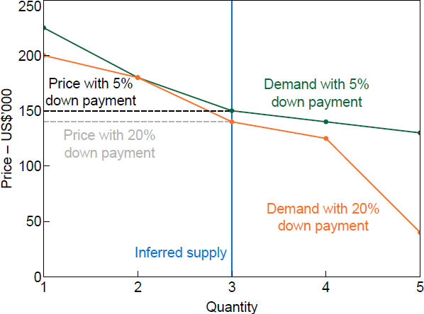
I can describe the experimental data and illustrate my analytical technique with an example. In the data there are five households from Michigan that live in a home valued at US$140,000. The households are asked to imagine a hypothetical situation in which they are moving to a different town and have found a home they like that is similar in value to their current home. They are then asked how much they would be willing to pay for the house given they need a 20 per cent down payment and can use a loan for the balance of the price.[1] The five responses range from US$40,000 to US$200,000. As long as each household demands at most one dwelling to live in, the WTPs ordered from highest to lowest form a market demand curve that shows demand for homes at any given price. Figure 1 shows this demand curve, as well as the demand curve with a 5 per cent down payment required, constructed in the same way.
As expected, the looser collateral constraint shifts the demand curve outward, but the shift is not uniform. Demand at the upper end barely shifts from the baseline 20 per cent down payment to the looser requirement of 5 per cent. At the lower end of the demand curve, the shift in demand is much larger. This pattern is consistent with constraints binding more at the lower end of demand. As the constraint is loosened, these households responds by raising their WTPs.
Translating these demand curves into a price change requires a supply curve. The supply curve is not observable but it must intersect the demand curve at the price, which is available in the data as the estimated home value. I illustrate the price effect using a vertical supply curve that intersects the demand curve with tighter constraints at the market price. The change in price can then be determined as the change in the marginal WTP. In the example in Figure 1, the average change in WTP is US$28,000 while the change in the marginal WTP is US$10,000.
Sources: Author's calculations; Fuster and Zafar (2021)
The rest of the paper shows how this same pattern seen for US$140,000 homes in Michigan is borne out in the aggregate data and within most market segments. Constrained households have low WTPs, typically below the marginal WTP, and tend to respond most to collateral constraints. As a result, the average change in WTP is greater than the change in the marginal WTP. For the average change in demand to equal the change in price the shifts in demand would need to be even across the curve.
Analysing the demand curves across the full dataset in Fuster and Zafar (2021) follows the same principle as the above example, but is complicated by aggregation. The relatively small size of the survey means it is not feasible to recreate local housing markets in detail. To analyse the full dataset I aggregate household demand for homes of different values in different locations. In aggregate, my estimate of the change in market price caused by a loosening of collateral constraints is a 6 to 8 per cent increase compared with the average WTP increase of 16 per cent reported in Fuster and Zafar (2021). Analysing disaggregated subsets of the data shows the same pattern. Within each segment, more-constrained households tend to have low WTPs that have little effect on prices despite their larger responses to looser collateral constraints.
For the mortgage rate cut experiment, analysing the demand curves does not show systematic differences between the average effect of interest rates and the effect on the marginal buyer. This demonstrates that the collateral constraint result is not an artefact of the method, and also makes sense in the context of the experiment. There is no servicing constraint in the experiment so a changing mortgage rate does not change any constraint. As such, there is less reason to expect a different effect across the demand curve.
To help interpret the results of the empirical analysis of the demand curves, I consider a heterogeneous-agent user cost framework. In this framework households vary in their subjective discount rate and their relative preference for renting versus owning a home. These two preference parameters can be identified from the survey data because they jointly determine the level of a household's WTP and the response to a change in collateral constraints. A household with a relatively steep discount rate will have a lower WTP and respond more to a change in constraints. A steep discounter with a strong preference for owning over renting will have a high WTP and respond strongly to collateral constraints, but such households are rare in the data.
I estimate empirical models that show a household's survey responses can, to some extent, be predicted from observable household characteristics. Using only the predictable variation in survey responses to constructing housing demand curves gives similar results to the raw data. This prediction exercise shows that the systematic variation in household behaviour based on observable characteristics is an important source of heterogeneity that can drive market outcomes. Similar household characteristics are available in a variety of standard data sources, which allows me to use the experimental findings to infer the sensitivity of housing prices to financing conditions in other times and places. I validate my out-of-sample method using an independent contemporary data source for the United States and then apply the method to other datasets. Applying the model to Australian data suggests that the effect of collateral constraints is similar to in the United States, and has not changed substantially over the past 20 years. The model implies somewhat different effects in countries with much higher or lower rates of home ownership.
The marginal buyer sets the price in asset markets. This paper shows that in housing markets, collateral constraints have meaningfully different effects on average, compared with the effect on the marginal buyer. There are few empirical attempts to understand how heterogeneity in markets can lead the marginal buyer to diverge from average changes, in part due to the rarity of this kind of detailed data.[2] The method I employ may be useful in a wider range of empirical analyses, and can also help clarify divergent results in the housing modelling literature. Many housing models include heterogeneity, and show very different effects of collateral constraints on price. For collateral constraints to have a large effect on prices, constrained buyers must be marginal. My analysis gives reasons to think that this is relatively rare.
For policymakers assessing the effects of macroprudential policy, this paper shows that using average effects of collateral constraints on households is likely to overstate the effect on market prices. My results reinforce other recent literature on the importance of household heterogeneity in the transmission of macroprudential policy. Further, I show that the effects of constraint changes depend on the market structure and household characteristics that can vary over time and place.
The next section reviews the literature on the role of collateral constraints in housing markets, with a focus on heterogeneity. After that I further explain the method used to estimate the change in WTP of the marginal buyer, and apply it to the aggregate experimental data and a range of market segments. I then describe a heterogeneous user cost model that can interpret the empirical features of the data, before estimating regression models and using them to simulate the response of housing markets to changing collateral constraints using standard household survey data from other sources, including the Australian Survey of Income and Housing. Finally, I conclude with the implications for housing market models and policymakers.
2. The Role of Collateral Constraints is Contested
The effect of collateral constraints has been studied extensively in the context of the US housing boom and bust. More recently, collateral constraints in the form of loan-to-valuation (LTV) ratio limits have been the subject of research into macroprudential policy assessment. Part of the difficulty in figuring out cause and effect is that financing conditions vary endogenously with price expectations and many other variables. The experiment in Fuster and Zafar (2021) overcomes this difficulty by providing exogenous variation, at the cost of using stated preference responses rather than actual behaviour.
Across literature on both the US housing boom and macroprudential policy, the importance of household heterogeneity has become increasingly recognised. This paper finds that the effects of collateral constraint on prices depend crucially on household heterogeneity through its effect on the responsiveness of housing demand to credit constraints across the demand curve. There is no reason to expect the overall effect of credit constraints to be consistent over time or in different markets, which may explain some of the disagreement in the existing literature.
2.1 Collateral constraints in the US housing boom
Early research into the housing boom and bust in the United States attributed an important causal role to relaxed lending standards and collateral constraints. In the empirical micro literature, Mian and Sufi (2009) document that zip codes with more subprime borrowers in 1996 had disproportionately high mortgage growth in the boom and default rates in 2007 in the United States. They note that the expansion of credit in the 2002–2005 period was concentrated in areas with relatively low income growth. This was taken as evidence that the housing boom was caused by a credit supply shock enabled by increased securitisation. More recently, Foote, Loewenstein and Willen (2016) show that by looking at originations, rather than debt stocks, Mian and Sufi (2009) mistook a relative increase in turnover in low-income places for an increase in credit. Adelino, Schoar and Severino (2016) use loan-level data to show that there were large increases in credit in middle-income and prime borrowers. They argue this opposes the view put forward in Mian and Sufi (2009). Mian and Sufi (2017) argue that the income measure used in Adelino et al (2016) was artificially inflated due to fraudulent income reporting on mortgage applications, while tax data show that income growth amongst households with strong credit expansion was weak. Albanesi, De Giorgi and Nosal (2017) use individual-level data to show that almost all of the disproportionate growth in subprime zip codes can be explained by life-cycle effects as households in these zip codes aged. Further, prime borrowers in these zip codes also showed strong growth in mortgage debt.
The macro modelling literature is equally divided. Two recent prominent papers reach essentially opposite conclusions. Favilukis, Ludvigson and Van Nieuwerburgh (2017) use a model to attribute the boom and bust in US housing prices largely to changing collateral constraints. Kaplan, Mitman and Violante (2020) argue that the conclusion in Favilukis et al (2017) relies on unrealistic modelling assumptions, including one-period mortgages that are subject to refinancing risks and an absence of a rental market. The model in Kaplan et al (2020) makes more realistic assumptions about renting and mortgage markets, and attributes little of the price swings to collateral constraint changes. Empirical VAR studies also give conflicting results. Cox and Ludvigson (2021) attribute price swings to collateral constraints whereas Ben-David, Towbin and Weber (2019) attribute them to expectations.
2.2 Assessment of macroprudential policy
Changing the maximum allowable LTV ratio on housing loans is one common tool of macroprudential policy. Most research on LTV caps shows some dampening effect on prices and credit, but progress on estimating the size of the effects has been more difficult. In one recent example, Richter, Schularick and Shim (2019) use narrative identification and inverse propensity-weighted local projections to estimate the magnitude of the effect of LTV restrictions on housing prices in an international panel. They find a typical LTV tightening lowers prices by 1.5 per cent over the following year, growing to 8 per cent over four years. That is the average finding, with the effect larger in emerging economies and smaller in advanced economies.
Research on LTV caps has, to some extent, considered the heterogeneous effects on different households. Van Bekkum et al (2019) find that LTV caps have larger effects on the borrowing of constrained households, while Acharya et al (2020) find loan-level lending constraints tend to reallocate credit from low-income to high-income households. Armstrong, Skilling and Yao (2019) use the differential application of collateral constraint policy on existing and new houses to estimate a dampening effect of the policy on prices, although they find the effect depends on other factors such as the pace of recent house price growth.
As pointed out in Duca, Muellbauer and Murphy (2021), time series analysis of macroprudential policies in general, and LTV policies in specific, is made difficult by the endogeneity of policy actions, and the tendency for policymakers to coordinate different policy levers. The stated preference approach can introduce genuine exogeneity.
2.3 Household heterogeneity is important when considering collateral constraints
Several previous modelling studies have looked at heterogeneous responses of households to changes in collateral constraints. Saver–spender models of the housing market, such as Iacoviello (2005) and Justiniano, Primiceri and Tambalotti (2019), have two types of agents. The patient agent is unconstrained and their housing demand does not respond at all to changing collateral constraints, while the impatient agent is constrained and their housing demand responds substantially to collateral constraints. The actual effect on prices depends on the structure of the model, in particular market segmentation and the rental market (see Cusbert (2022) for details).
The model of the San Diego housing market in Landvoigt, Piazzesi and Schneider (2015) models richer household heterogeneity and takes the housing stock to be of varying quality over a continuum. In effect this means the housing market is partially and continuously segmented. Each buyer is marginal in its own segment, but there are spillovers between segments. There is no rental market in the model, which makes each household a marginal buyer. Household heterogeneity creates differing responses to collateral constraints, which flow through to price. Overall, they find the bottom quintile of housing prices respond relatively strongly to easing credit constraints.
Kaplan et al (2020) model households with heterogeneous responses to collateral constraints and the option to rent instead of own housing. Similar to Landvoigt et al (2015) and Justiniano et al (2019), only constrained households respond much to collateral constraints. But unlike in those models, in Kaplan et al (2020) the households who respond to collateral constraints are not typically marginal buyers so the effect on price is minimal.
The experimental approach allows a more direct empirical analysis of the interaction of household heterogeneity with collateral constraints that is less dependent on a particular model structure. The analysis in Fuster and Zafar (2021) shows heterogeneous responses to collateral constraints based on household characteristics, which is consistent with the models mentioned in this section. But as shown by the differences in results of the models discussed, heterogeneous responses to constraints is not sufficient to infer what happens to prices. This paper considers the heterogeneous response of households in the context of the market structure to explicitly estimate the changes in marginal buyer demand and thus prices. Broadly speaking, my results for the response of housing prices to collateral constraints are are closer to the zero response of Kaplan et al (2020) than the large responses in Landvoigt et al (2015) and Justiniano et al (2019). That said, the marginal buyer does show a significant response to credit constraints in the survey data. Households that respond most strongly to collateral constraints are not typically marginal, but marginal buyers appear to be somewhat constrained. The direct empirical analysis highlights that households seem to be constrained along a continuum rather than being classified as constrained or unconstrained.
3. The Survey Experiment
The stated preference survey experiment was appended to the US Survey of Consumer Expectations (SCE) run by the New York Federal Reserve Bank in 2014. This ensures both a representative sample and a rich set of financial data to add to the survey responses. The respondents were asked for their WTP for a home under four different conditions. Full details of the questions are available in Fuster and Zafar (2021),[3] and a summary is as follows.
- The respondent is asked for an estimate of the value of the home they currently live in, among other questions about household characteristics.
- Scenario setup: You are moving to a new city, and want to buy a house to live in for the indefinite future. You find a home you like; similar homes have been selling for <insert respondent's estimate of home value>. If the respondent owns their home, the scenario states that they sell it and discharge their mortgage.
- Question: Suppose you need a down payment of 20%, and the mortgage rate is 6.5%. How much are you willing to pay for the home, bearing in mind you need to be able to make the down payment?
-
Repeat question for:
- Minimum down payment of 5%,
- Mortgage rate of 4.5%, and
- Inheritance of US$100K.
Fuster and Zafar (2021) report that most respondents spent some time using the provided repayment calculator to assist with the decision. The main results in Fuster and Zafar use the unweighted SCE sample, although they show that using the sample weights makes little difference. For comparability with the main results I do not use weights.
4. Method: Finding the Marginal Buyer on the Demand Curve
My aim is to consider the change in the WTP of the marginal buyer between each pair of experimental conditions. To identify the marginal buyer, I aggregate responses to construct a demand curve in each experimental condition. The marginal buyer need not be the same person before and after the change in conditions. Combined with an inferred supply curve, the pair of demand curves allows me to locate the marginal buyer in each condition and determine the price change between conditions.
The WTP data is for owner-occupied housing, which means that each household demands either one or zero houses at a given price. Total market owner-occupier demand at any price is thus given by the number of respondents with a WTP equal to or greater than that price. Fuster and Zafar (2021) assume fixed supply in their representative agent user cost framework. I do the same here, both to make my results comparable with theirs, and to provide an upper bound on price changes.[4]
To construct the market demand and supply schedules, I follow the same procedure as the illustrative market segments with an extra initial step to allow comparison across different home values:
- Take the ratio of the WTP to the home value (I term the result the ‘normalised WTP’).
- Order the normalised WTPs from highest to lowest to show the number of households that will buy at any given price. This forms a demand curve, which can also be thought of as the reverse cumulative distribution function for the normalised WTPs. Applying this step to the 20 per cent down payment baseline condition and the 5 per cent down payment loosening condition shows the outward shift in the demand curve.[5]
- Infer the location of the vertical supply curve from the intersection of one of the demand curves with the home value. For normalised WTPs this is always 1 (or zero in logarithms).
- Find the intersection of the shifted demand curve with the supply curve to determine the price change.
Fixed supply is typically considered as a limited building response rather than inelastic supply of existing houses for resale (see Cusbert (2022)). However, because housing demand in the Fuster and Zafar (2021) approach only accounts for owner-occupiers, supply also includes any houses owned by investors in the baseline condition. The assumption of unresponsive supply means investors do not change the number of houses they own in response to the change in credit conditions. There are two interpretations of this assumption. One is that investors are completely inelastic, and none buy or sell in response to the change in credit conditions or increase in demand. Alternatively, investors could be price elastic and also respond to the easing in credit conditions by increasing the price at which they are willing to sell. If these two effects offset to maintain the number of houses owned by investors, it is equivalent to constant supply.
The experimental data cannot inform the behaviour of investors, and other studies suggest the characteristics of investors vary substantially in different circumstances and over time. Graham (2020), Greenwald and Guren (2021) and Cusbert (2022) explore in detail the consequences of different investor behaviour for price and ownership structure. Broadly speaking, investors that are more price elastic dampen the price response, while investors that are more reliant on credit boost the response. The lack of information about investors is a limitation of the experimental dataset that is worth bearing in mind. I maintain the simple assumption of constant supply from Fuster and Zafar (2021), which maintains the focus on the structure of heterogeneity in the owner-occupier demand curve.
5. Aggregate Results
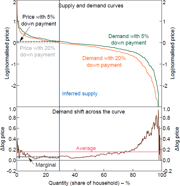
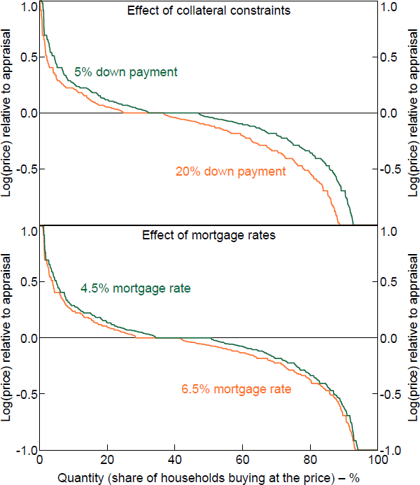
Comparing demand curves before and after the easing in collateral constraints reveals a clear pattern in the data (Figure 2). The upper end of the demand curve, with higher normalised WTPs, does not shift much while the lower end shifts substantially. The top panel of Figure 2 shows the demand curve constructed for each experimental down payment condition. Each demand curve shows the quantity demanded, on the horizontal axis, as a function of price on the vertical axis. The quantity is expressed as a share of total households in the sample because the raw number in the sample is not meaningful and there is no specific housing market that we are thinking about. The price is expressed relative to the home value, which allows the aggregation of WTPs from households who live in homes of different values, as outline in the method in Section 4. The figure shows the logarithm of the normalised price so shifts in demand can be interpreted as multiplicative changes (or approximate percentage changes). The lower panel shows just the shift in demand, which makes the pattern easier to see and highlights the difference between the average change and the change in the marginal buyer.
Table 1 shows my central estimates and bootstrapped confidence intervals for the change in the WTP of the marginal buyer (i.e. the price) assuming inelastic supply, and compares them to the average change in WTPs.[6] The WTP of the marginal buyer rises by around 6 per cent when collateral constraints are eased, which is significantly less than the 16 per cent average rise in WTPs. The pattern of the shift in demand curves and the difference between the average effect on WTPs and the effect on the marginal buyer are consistent with the idea that households who respond most to collateral constraints tend to have WTPs that are too low to affect the market price.
Note: The normalised price is relative to the home value given in the survey data.
Sources: Author's calculations; Fuster and Zafar (2021)
| Looser collateral constraint | Lower mortgage rate | Inherit US$100,000 | |
|---|---|---|---|
| Average WTP change | 0.16 (0.14–0.18) | 0.04 (0.04–0.05) | 0.11 (0.09–0.13) |
| Change in marginal WTP | 0.06 (0.04–0.08) | 0.05 (0.03–0.06) | 0.07 (0.06–0.10) |
| Difference | 0.10 (0.07–0.12) | 0.00 (–0.02–0.10) | 0.04 (0.03–0.07) |
|
Notes: Data are trimmed at 5 per cent based on (WTP) in each experiment, as in Fuster and Zafar (2021). Respondents with WTP equal to home value in either of the scenarios are excluded for each experiment (see Appendix B.3 for details). |
|||
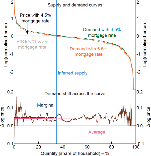
I compare the demand curves before and after the interest rate change using the same method. In this case, there is not much of a pattern across the demand curves with a higher interest rate compared to the demand curve with a lower interest rate (Figure 3). There is no systematic relationship between the change in WTP and the location on the demand curve, and consequently there is no difference between the change in the marginal buyer's WTP and the average change.
There was no debt-servicing restriction in the experimental questions, so changing the mortgage rate does not relax any hard constraints. As such there is no real reason to expect a systematic relationship between the shift of the demand curve across the market. Fuster and Zafar (2021) report that the interest rate effect is on the lower end of the range of empirical estimates, and that the uncertainties in how survey respondents interpret the effect on the term structure make the result a bit hard to benchmark. Further, if survey respondents are taking the interest rate cut as applying only to them, these results may miss an amplifying general equilibrium-type of effect that would operate through the home value (see Appendix A.1).
Note: The normalised price is relative to the home value given in the survey data.
Sources: Author's calculations; Fuster and Zafar (2021)
The average effect of the collateral constraint change is much larger than the average effect of the interest rate change, as reported in Fuster and Zafar (2021). But viewed through the lens of the marginal buyer method, the effects of the two changes have similar magnitudes.
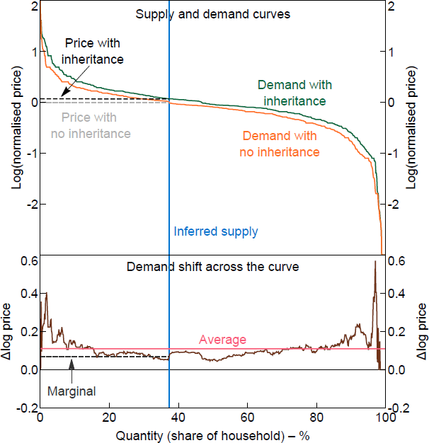
The demand curves for the inheritance experiment show more of a pattern than the mortgage rate experiment, but less than the down payment experiment (Figure 4). Constrained households are likely to have their constraints eased by the inheritance, which might suggest it should have the same structure as the down payment scenario. On the other hand, the inheritance can be used for anything – there is no guarantee a respondent would choose to put it toward a home.
Note: The normalised price is relative to the home value given in the survey data.
Sources: Author's calculations; Fuster and Zafar (2021)
6. Market Segments and Aggregation
In aggregate there is a clear relationship between the size of a household's response to loosening collateral constraints and its position on the demand curve. The large responses that drive up the average are typically from households with low WTPs that have no bearing on the market price. In practice, this aggregate market does not exist so it is worth considering whether it is a reasonable reflection of any given housing market. Disaggregating the data also shows how collateral constraints can have different effects in different housing markets.
A possible concern is that by aggregating the data I am obscuring different market outcomes in different housing market segments. For example, there could be some segments in which the marginal buyer is constrained and responds strongly to credit constraints compared to the average response in that segment. If that were the case, there would be no guarantee that the marginal buyers in those segments would have much influence over the estimate of the marginal buyer in aggregate. Looking at more disaggregated data suggests that different market segments do differ in their responsiveness to collateral constraints. However, the pattern observed at the aggregate level is also evident at disaggregated levels. Within every segment I analyse, the change in the marginal buyer's WTP is less than the average change.
The value of a home is one important dimension of market segmentation. This was a focus of Landvoigt et al (2015), which found that in response to an easing of credit conditions, the prices of cheaper homes increased by more than the prices of more expensive ones. The structure of the model in Landvoigt et al (2015) makes all households marginal by assumption, even though they find that constraints appear to bind differentially for households with similar housing demand. For example, a young household with a high income and low wealth may target similar housing to an older household with higher wealth and less binding constraints.
To examine market segmentation by home value, I look at each quintile of home values separately. Table 2 shows that households in the lower quintiles of homes are more commonly renters and tend to have less available equity as a proportion of their home value. Conversely, age and normalised WTP in the 20 per cent down payment condition are similar across quintiles.
| Value quintile |
Mean | Median | ||||||
|---|---|---|---|---|---|---|---|---|
| Home value (US$′000) | Age | Normalised log(WTP20)(a) | Equity available(b) | Normalised log(WTP20)(a) | Equity available(b) | |||
| 1 | 72 | 46 | −0.35 | 0.91 | −0.16 | 0.19 | ||
| 2 | 135 | 47 | −0.42 | 1.11 | −0.11 | 0.51 | ||
| 3 | 188 | 45 | −0.27 | 0.80 | −0.12 | 0.40 | ||
| 4 | 284 | 50 | −0.47 | 0.94 | −0.15 | 0.60 | ||
| 5 | 538 | 50 | −0.51 | 1.08 | −0.21 | 0.90 | ||
| Total | 236 | 48 | −0.40 | 0.96 | −0.15 | 0.48 | ||
|
Notes: (a) Log of WTP with 20 per cent down payment divided by home value. Sources: Author's calculations; Fuster and Zafar (2021) |
||||||||
To look at the effects of this household heterogeneity, I calculate the average WTP change and the change in the marginal buyer's WTP, treating each quintile as a market segment and using the same method as above to estimate the change in the marginal buyer's WTP. Figure 5 shows my results in comparison to the average price response in each quintile as reported in Landvoigt et al (2015). In both sets of results the lower quintiles are more responsive to easier credit conditions. In my results, however, there is also heterogeneity within each quintile that means the change in the marginal buyer's WTP is less than the average change. There is much more heterogeneity in the effect of the collateral constraint than the mortgage rate, both within and between quintiles. Lower heterogeneity for the mortgage rate response is consistent with the lack of systematic variation in the response of WTPs to the mortgage rate in the aggregate demand curve analysis.
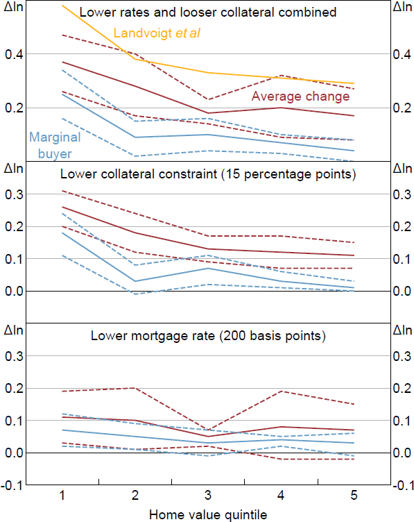
Note: Dashed lines represent 95 per cent confidence intervals.
Sources: Author's calculations; Landvoigt, Piazzesi and Schneider (2015, Figure 10 panel B)
There are many other demographic, location and financial variables that could be important factors in market segmentation, although they are less likely to map to a literal housing market (Figure 6). Analysing subsamples separately weakens the aggregation assumptions required for the main results, although the smaller sample sizes increases the width of the confidence intervals. Overall, the point estimate of the change in the marginal buyer's WTP is smaller than the average change in all segments examined, and the 95 per cent bootstrapped confidence interval for the difference between the two does not contain zero in any segment. For segments in which the average effect is relatively low, the differences between the two methods tend to be small.
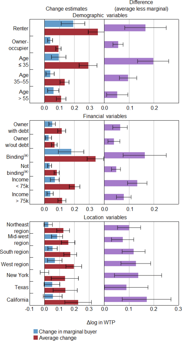
Notes:
Whiskers show 95 per cent confidence intervals.
(a) A down payment is binding if the household's wealth available for a deposit is less than 20 per cent of the home value.
Most segments either display a non-parallel shift in demand, with bigger shifts at the lower end, or very little shift in the demand curve. The first pattern is seen in segments where constraints are more likely to bind, like a segment of younger households (Figure 7, left panels). Average effects are large and the change in the marginal buyer is significantly lower. The second pattern is seen in segments where constraints are unlikely to bind, like homeowners with no debt (Figure 7, right panels). Average effects are small and the change in the marginal buyer WTPs are even smaller.
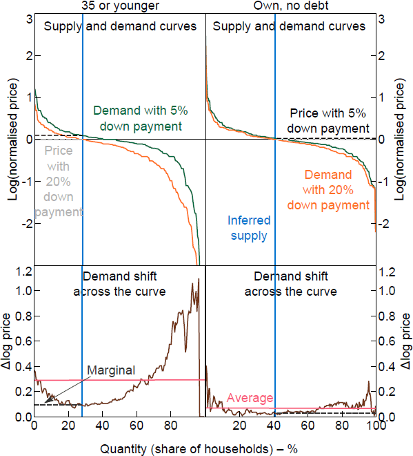
Note: The normalised price is relative to the home value given in the survey data.
Sources: Author's calculations; Fuster and Zafar (2021)
7. Robustness Checks
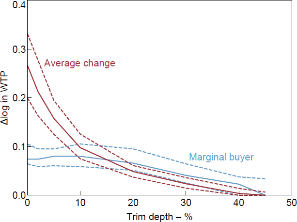
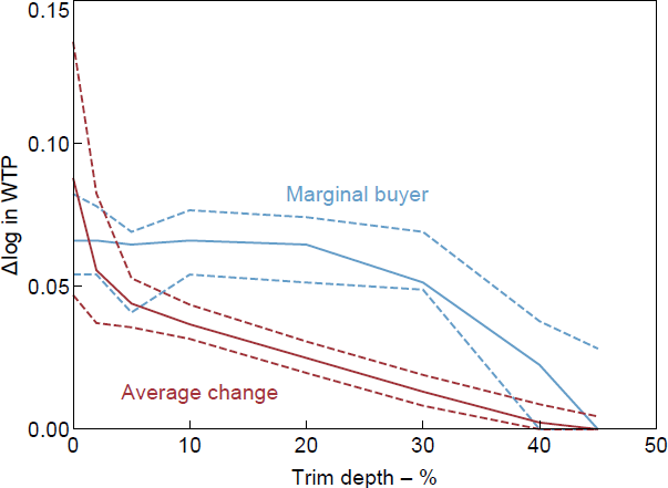
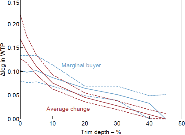
The amount of data trimmed and the treatment of WTPs exactly equal to the home value affects some of the estimates of the main results. Some trimming is required because the data are from a stated preference experiment and likely include outliers, either because of errors filling in the form or inattention. But the skew in the data appears to reflect genuine heterogeneity, so trimming too much will remove important variation that should inform the central estimate. The results presented above trim out 5 per cent of the data by the log change in WTP as in Fuster and Zafar (2021). Appendix C.2 shows that the estimate of the average change in WTP is quite sensitive to the trim depth but the estimate of the change in the marginal buyer's WTP is not.
In each experimental condition, some respondents give WTPs exactly equal to the home value. Translating this to a demand curve means there is a flat area of the demand curve at the market price, which means the supply curve could intersect the demand curve anywhere in that area (Figure B5). There are three reasons why I exclude some of these WTPs. First, some respondents may interpret the home value as a ceiling for a reasonable WTP. The respondent is told the amount that similar homes are selling for. If they assume they could buy an equivalent house for that price, it would not make sense to pay more for one particular house. Clearly not all respondents answer in this way, so removing any who do is useful. Second, the flat area in the demand curve means the supply curve, and thus the price change, is indeterminate and can lie in a relatively broad range. Third, including the flat area typically lowers the estimate of the change in marginal buyer WTP and has a negligible effect on the mean.
For the main results, I discard WTPs exactly equal to the home value in either experimental condition of the comparison. Appendix B.3 shows that different treatment of WTPs equal to the home value has little effect on the results of the collateral constraints experiment but does affect the results for the interest rate and inheritance experiments. The collateral constraint experiment has the largest, most reliable, and most statistically significant difference between the average WTP change, as reported in Fuster and Zafar (2021), and the change in the marginal buyer's WTP that determines the price change.
8. Interpreting the Experimental Results with a User Cost Model
The non-parametric demand curve analysis used above estimates the effect of financing conditions on the marginal buyer's WTP, and shows the difference between it and the average WTP change. But it cannot say much about the why the marginal buyer and the average diverge. My explanation is that more responsive households are responsive because they are more constrained and have WTPs below the market price, which means they are less likely to bear on the market price. The user cost model of housing demand, presented in Fuster and Zafar (2021) and adapted here for heterogeneity, can give a more precise description of the mechanisms involved.
8.1 Standard user cost model
Fuster and Zafar (2021) consider the response of WTPs to the easing of collateral constraints through the lens of a standard user cost model as set out in Glaeser, Gottlieb and Gyourko (2012) and reprinted below as Equation (1). The idea of the user cost model is that a household compares the present value of the costs of renting a home and buying the same home, then chooses whichever is cheaper. For the marginal buyer, the costs of renting and buying should be equal in equilibrium, which means the user cost as a fraction of price should equal the rent-to-price ratio.
: down payment fraction
: subjective discount rate
: mortgage rate after tax deduction, where is marginal tax rate
: property taxes, maintenance, insurance (as a fraction of price)
g : growth rate of rent
: mobility rate.
Assuming fixed rent and supply, Fuster and Zafar (2021, p 237) note that ‘the elasticity of the equilibrium price thus corresponds to the elasticity of demand, which is what we will measure in our survey’. They measure average elasticity, but the elasticity of the marginal buyer determines price changes. These will coincide if all market participants have the same elasticity, but the heterogeneity in responses shows that is not the case. Fuster and Zafar do report different average elasticities within subgroups – most notably renters versus owners – but as demonstrated by the analysis of market segments in Section 6 households within segments show important heterogeneity and the elasticity of many individuals' demand is irrelevant to market pricing.
8.2 A heterogeneous user cost model
Recognising that not all WTPs influence market pricing calls for a slightly altered heterogeneous user cost model. I adapt the standard user cost framework to include an idiosyncratic discount rate for each household, i (Equation (2)). Relaxing the representative agent assumption breaks the direct mapping from demand to price, so the equation is now specified as a WTP for each household rather than the price. Further mapping to the price requires considering who is marginal.
The subjective discount rate is an important dimension of heterogeneity but is unlikely to be the only one, and it cannot account for all the variation in the data. In principle, any element of the user cost model can be heterogeneous. Previous modelling research on the rent versus buy decision often includes a rental preference parameter, for example, Corbae and Quintin (2015), Kaplan et al (2020) and Greenwald and Guren (2021). To keep the model simple and engage with that literature, I add a rent versus own preference parameter, , to the user cost model. For > 0 the household is willing to pay more than the discounted sum of rent to own the house, and vice versa for < 0. For all other parameters in the user cost equation I use the calibration from Fuster and Zafar (2021).
Conditional on the calibrated cost parameters, Equation (2) shows how the preference parameters determine both the ratio of a household's WTP to the rent on a home, as well as the elasticity of the WTP to a change in collateral constraints. The level of the WTP is determined by both the rent versus own parameter, , and the subjective discount rate parameter, . The response to collateral constraint changes is determined only by because WTP is linear in . Figure 8 shows the WTP-to-rent ratio as a function of , assuming = 0 (i.e. indifference between owning and renting), a before-tax mortgage rate of 5.5 per cent, and using the Fuster and Zafar (2021) calibration for the cost parameters.[7] The WTP is steeply decreasing in as the household increasingly discounts the value of future imputed rents.
The lower panel of Figure 8 shows the response of a household's theoretical WTP to the experimental changes of loosening the collateral constraint and cutting the interest rate. The response of WTP to collateral increases sharply in . If a household's subjective discount rate is equal to the after-tax mortgage rate (3.6 per cent in this example), then the WTP response is zero, climbing to a log change of 0.3 at a discount rate of 20 per cent. The response of WTP to a change in interest rate is little changed across the spectrum of subjective discount rates.
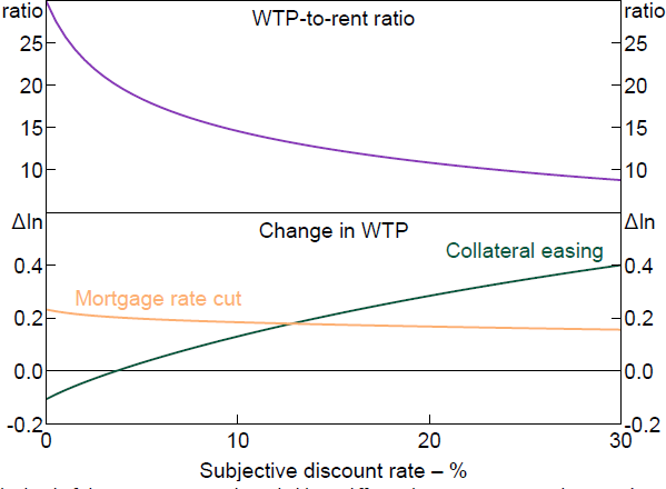
Note: The level of the WTP assumes a household is indifferent between owning and renting (i.e. = 0), while the change is independent of .
The heterogeneous discount rate is written in Equation (2) as a preference parameter, but it can be thought of as combining genuine preference heterogeneity with differences in circumstances. The key circumstance is likely to be the household's available financial resources compared to the collateral required for their home. That said, household preferences are likely to affect accumulation of financial resources, which makes it difficult to disentangle preferences and circumstances without a more detailed model. To avoid taking a stand on the behavioural mechanism and let the experimental data speak for itself, I combine circumstances and preferences into one parameter. Similarly, the rent versus buy parameter is likely to be influenced by life-cycle factors as well as deeper preferences.
8.3 Mapping the data to the heterogeneous user cost model
The heterogeneous user cost equation in Equation (2) creates a mapping from the WTP data onto the discount rate and rent versus buy preference parameters. A similar approach was taken in Alvarez and Argente (2020) to model heterogeneity in a very different experimental setting about using cash for payments. For the Fuster and Zafar (2021) experiment, each WTP question for each household gives an instance of Equation (2) with different values for WTPi , and r. From there, the equations can be solved for the preference parameters, and , for each household.[8]
Equation (2) also includes the rent of each dwelling, which is not observed. The discount rate, , can be identified from the ratio of WTPs in the two down payment scenarios, which means it does not depend on rent. Because a household's WTP is linear in the rent versus own preference parameter, , it cancels out within the ratio. Identifying does require the rent of each dwelling. To proxy for rent, I multiply the home value by the rent-to-price ratio implied by the Fuster and Zafar (2021) calibration of the user cost model with the discount rate equal to the mortgage rate.
Figure 9 shows a scatter plot of the joint distribution of the preference parameters inferred from the WTP data overlaid on the theoretical relationship of the two parameters with the level of WTP.[9] With two dimensions of heterogeneity it is possible for households with a high initial WTP to be very responsive to changes in down payment restrictions. Such a household would have a high discount rate, , possibly due to financial constraints, and a strong preference to own rather than rent. This region of the preference space corresponds to the lower right region of Figure 9. A market segment including many households within this region would exhibit both a responsive marginal WTP and a responsive average WTP. In the data this area is sparsely populated, which is consistent with the direct analysis of demand curves – the large increases in WTP are mostly at the lower end of the normalised WTP spectrum in levels.
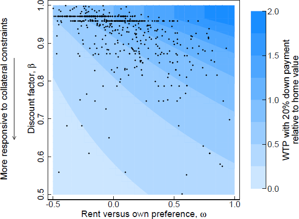
Notes
The contours in the figure show the theoretical relationship between WTP and the preference parameters with 20 per cent down payment. Each dot shows the preference parameter inferred from a household's WTPs.
(a) I transform the interest-rate-equivalent subjective discount rate to a subjective discount factor They can be used equivalently in the user cost model but is easier to visualise because WTPs close to zero map to values close to zero and values approaching infinity.
Sources: Author's calculations; Fuster and Zafar (2021)
9. Empirical Model: Simulating Demand Curves from Household Characteristics
Empirical modelling reveals that some of the heterogeneity in households' WTP responses can be predicted based on observable household characteristics like income, wealth, age and housing tenure status. Further, this predictable component of heterogeneity is sufficient to drive the differences between average changes in WTPs and the change in the marginal buyer's WTP observed in direct analysis of the demand curves. This finding complements the theoretical user cost approach by showing that the pattern of heterogeneous behaviour in the survey can be quantitatively explained by observable household characteristics.
The empirical models can also be used with observational datasets that do not include stated preference questions for out-of-sample inference about the effect of financing conditions. I show that the estimated effects are similar using US data from the Survey of Consumer Finances, and then simulate the effects of financing conditions in other times and countries.
The relationship between a household's discount rate and their WTPs in different financing conditions is nonlinear (see Figure 8). In principle, mapping the empirical model through the user cost framework could improve upon a simple linear model of WTP as a function of household characteristics. However, the nonlinearity is only important for very steep discounters, and the predictions models do not capture that part of the distribution well (see Appendix C.1 for details). As a result, I focus on the simple OLS models because they work at least as well as the user cost model when taken to the data, the marginal effects are easier to interpret, and they do not require normalisation.
9.1 Leave-one-out prediction method
Simulating demand curves requires predictions of the normalised WTPs in both down payment conditions, generated from observable financial and demographic variables. Fuster and Zafar (2021) estimate regression models with a large set of observational variables that do just that. My focus is on prediction, including out-of-sample prediction, so I guard against overfitting in two ways. First, as well as replicating the estimations in Fuster and Zafar, I also estimate much smaller models. Second, I use leave-one-out predictions to assess the models and construct demand curves. For each household I estimate the parameters using all other households and then use the estimated parameters to construct a prediction for the household in question. Those predictions are used to calculate an R2 and construct the simulated demand curves.
I estimate linear regression models using Equations (3)–(7). Three different versions of the model use different explanatory variables, denoted X. The first is the full set of variables used in Fuster and Zafar (2021).[10] The second set is smaller and only includes variables that are important to behaviour and likely to be relevant in other time periods and places: tenure status (rent/own); age of the household head; as well as income and available equity, both expressed relative to the household's home value. The third set of explanatory variables is the same as the second but without tenure. Tenure drives a lot the variation in WTPs, but is quite correlated with other important variables like available equity. Removing it is helpful for investigating how the models work in other countries with different institutional arrangements.
where the and coefficient vectors for each household are estimated in regressions
To construct the demand curves I take the fitted values of the WTPs with two different collateral constraints from each of the leave-one-out regressions. I then order the WTPs using the same method as in the first part of the paper.
9.2 Results
The large model with the full set of explanatory variables has the best in-sample fit, but the fit worsens substantially using leave-one-out predictions (Table 3). Conversely, the small models have a similar fit in sample and using leave-one-out predictions, suggesting they are not overfitted and are more suited to out-of-sample predictions.
| X data used for predictions(a) | Full | Small | No tenure |
|---|---|---|---|
| Number of parameters | 50 | 5 | 4 |
| 0.21 | 0.16 | 0.11 | |
| 0.10 | 0.14 | 0.10 | |
| 0.26 | 0.22 | 0.16 | |
| 0.16 | 0.21 | 0.15 | |
| Mean (WTP) minus change in marginal WTP (0.11 in data) | 0.12 | 0.10 | 0.11 |
|
Notes: Outliers are removed by trimming 4 per cent from the dependent variables, in order to match the sample size of the 5 per cent trim of the change in WTP. |
|||
The simulated WTPs can be used to construct demand curves and model the change in the WTP of the marginal buyer. The mean change in simulated WTPs is the same as in the data by construction, but the method does not guarantee that the change in the marginal buyer's WTP matches the estimates directly from the WTP data. The bottom row of Table 3 shows that all the models are able to match the direct empirical estimate of the difference between the average WTP change and the marginal buyer WTP change. The systematic heterogeneity captured by the observable data is sufficient to drive the main results of demand curve analysis.
The two models with smaller sets of explanatory variables are the most promising models for out-of-sample simulation. Table 4 shows the parameter estimates for these two models for WTPs with a 20 per cent down payment, a 5 per cent down payment, and the change in WTP. Owning your own home is an important variable driving the effects of the collateral constraint. It raises the WTP in either down payment condition, but by much less in the looser per cent down payment condition. Similarly, available equity (relative to a household's home value) has a smaller positive effect on WTP in the looser condition. Owning a home is highly correlated with available equity, which means the coefficient on available equity is larger when tenure status is omitted. Available equity is inverse hyperbolic sine transformed to allow for households with zero and negative equity, while approximating a log-log specification for higher levels of equity.[11] To get a sense of the magnitude of the coefficient, the 0.10 for WTP20 means that a rise in a household's available equity from zero to 10 per cent of the home value leads to a doubling of its WTP, while a rise in available equity from 10 per cent to 20 per cent of the home value increases the household's WTP by 7 per cent. The income variable is inverse hyperbolic sine transformed in the same way. Income has the same positive effect on WTPs in both down payment conditions, so has no effect on the responsiveness to collateral constraints.
| WTP20% | WTP20% | WTP5% | WTP5% | (WTP) | (WTP) | |
|---|---|---|---|---|---|---|
| Owns home | 0.40*** (0.05) |
0.20*** (0.03) |
–0.20*** (0.03) |
|||
| Available equity(a) | 0.06*** (0.01) |
0.10*** (0.01) |
0.03*** (0.01) |
0.05*** (0.01) |
–0.03*** (0.01) |
–0.05*** (0.01) |
| Income(a) | 0.10*** (0.02) |
0.10*** (0.02) |
0.10*** (0.01) |
0.11*** (0.01) |
0.01 (0.01) |
0.00 (0.01) |
| Age(b) | –0.01 (0.01) |
0.01 (0.02) |
–0.03*** (0.01) |
–0.02 (0.01) |
–0.02** (0.01) |
–0.03*** (0.01) |
| Constant | –1.24*** (0.12) |
–1.18*** (0.12) |
–0.74*** (0.08) |
–0.71*** (0.08) |
0.50*** (0.08) |
0.47*** (0.08) |
| Observations | 816 | 816 | 816 | 816 | 816 | 816 |
| Adjusted R2 | 0.22 | 0.15 | 0.16 | 0.13 | 0.16 | 0.11 |
| RMSE | 0.51 | 0.53 | 0.35 | 0.36 | 0.32 | 0.33 |
|
Notes: ***, ** and * denote statistical significance at the 1, 5 and 10 per cent levels, respectively. Standard errors are in parentheses. (a) Available equity and income are relative to home value. |
||||||
Figure 10 shows the simulated demand curves for the smaller model including tenure status. As in the raw data, the shifts in demand are larger at the lower end of the demand curve. Overall the predicted demand curves are flattened compared to the raw data because idiosyncratic variation is driving the tails. The left panels show the simulation of conditional expected value for each WTP. The models only explain a fraction of the variation in the experimental data, which means the fitted values have less variation than the actual data. To better capture the variability of the actual data, the right panels of Figure 10 add stochastic idiosyncratic error terms for each household based on the estimated models. The error covariance is estimated using a seemingly unrelated regression system to capture the correlation of errors within an individual's response. The stochastic simulation better captures the spread of the data but misses the nonlinearity of WTP changes at the lower end of the demand curve.
The predicted demand curves contain only the systematic variation in responses. Any idiosyncratic variation among respondents, and any noise or errors from the survey, should be stripped out through the OLS estimation. In reality, both idiosyncratic and systematic heterogeneity among households will affect market pricing, but there is no way to reliably distinguish idiosyncratic heterogeneity from survey noise and errors.[12]
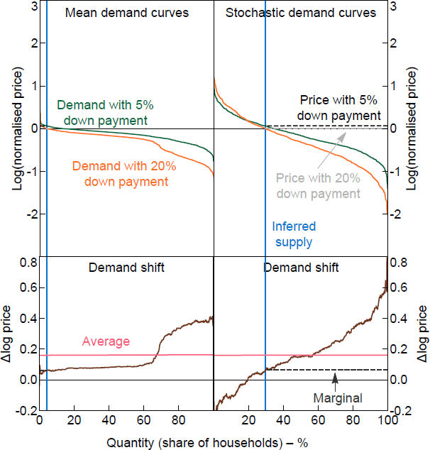
Notes: Mean curves show the fitted values for WTPs; stochastic curves add a random error generated using the error covariance matrix. The normalised price is relative to the home value.
9.3 Validating the model on contemporaneous US data
The estimated models above can be used to simulate stated WTP responses for any standard household data set that includes age, income, wealth, tenure status and home values.[13] As a validation exercise, I use the estimated models to simulate responses based on the US Survey of Consumer Finances (SCF) in 2013, which is an independent data source from the around same time as the survey used for the experiment. Figure 11 shows the simulated demand curves using the equivalent household characteristics taken from the 2013 SCF. The demand curves show a similar pattern to the demand curves from the SCE in Figure 10. As a result, the simulated average change in WTP and change in the marginal buyer's WTP are also similar across the two data sources, with the SCF simulations within 1 percentage point of the SCE results. The stochastic demand curves shown in the figures are one example of a stochastic draw of the demand curves simulated using the estimated error covariance matrix of the regressions. The mean demand curves are constructed from the conditional expected WTPs from the regression models.
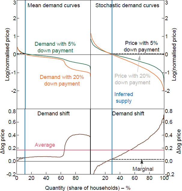
Notes: Mean curves show the fitted values for WTPs; stochastic curves add a random error generated using the error covariance matrix. The normalised price is relative to the home value.
Sources: Author's calculations; Board of Governors of the Federal Reserve System
9.4 Simulating the model with Australian data
In this section I take the estimated model and simulate the effects of a 15 percentage point loosening of collateral constraints using Australian data from the Survey of Income and Housing (SIH) between 2003/04 and 2019/20.[14] The US and Australian housing markets have some commonalities, like a owner-occupier rate of around two-thirds. The distribution of income, wealth and housing prices is different in the two countries, and that is what the simulation can take into account. Other differences in the housing market, and the mortgage market in particular, are not captured in the simulations. Two important differences are the tax deductibilty of mortgage interest in the United States, and the high prevalence of 30-year fixed, but refinanceable, mortgage rates in the United States compared to the use of variable rates and shorter-term fixed rates in Australia.
Home ownership is an important input to the model, and the rate of home ownership in the SIH fell from 72 per cent in 2003/04 to 69 per cent in 2019/20. There are notable differences between renters and owner-occupiers in home value, and even more so in available equity relative to a household's home value (Figures 12 and 13). Income relative to home value is much more similar across tenure status (Figure 14). Home value rises over time for renters and owners, while the distribution of income and available equity relative to home values are fairly stable over time.
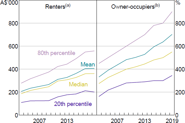
Notes:
(a) Imputed from reported rent and capital city rental yields.
(b) Self-reported.
Sources: ABS; Author's calculations
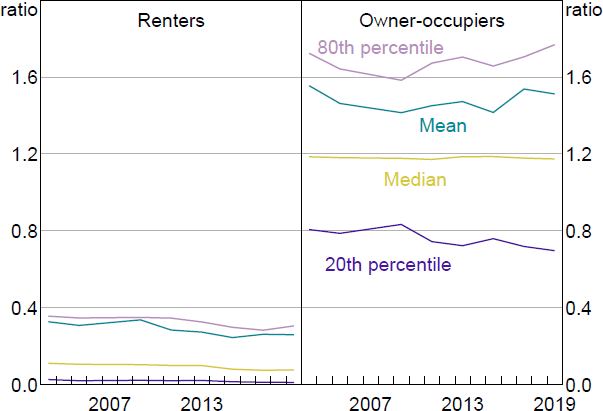
Note: Equity available is net wealth less superannuation, cars and trusts, divided by home value.
Sources: ABS; Author's calculations
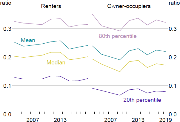
Sources: ABS; Author's calculations
The simulated responses of Australian households to an easing of down payment constraints based on the SIH input data are summarised in Figure 15.[15] All years show the same pattern as the actual US experimental data: the average WTP change is much greater than the change in the marginal WTP. Using the model including tenure status, the simulated average change in the Australian data is similar to the US experimental data at around a 15 per cent increase. Omitting tenure status attenuates the simulated effect in the Australian data but not the US. Omitting tenure status increases the simulated effects of observed wealth relative to home price, so the difference with the US results suggests Australian renters appear to be less constrained than US renters. The simulated change in marginal WTP is lower in the Australian simulations than the US data or simulations.
The simulation results for Australia are reasonably stable over time. Housing prices rose substantially between 2003 and 2019 but, as documented in La Cava and Wang (2021), household liquidity nevertheless increased. The simulated effects also take into account other forms of wealth, like home equity.
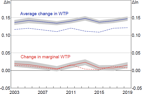
Notes: Solid line includes tenure status in the model; dashed line excludes. Shading denotes bootstrapped confidence intervals that show sampling variability from the Australian SIH data only.
To investigate the model simulations using different housing markets with different tenure arrangements, I apply it to Spain and Switzerland. These two countries have the highest and lowest home ownership rate in the OECD, respectively. In line with those home ownership rates, Spain shows a smaller effect of credit constraints than the United States and Australia, while Switzerland shows a larger effect. However, when tenure is omitted from the model, the differences in Spain and Switzerland are attenuated. Cultural and institutional differences related to the rent versus buy decision in those countries mean housing tenure is less correlated with financial constraints compared to the United States and Australia.
10. Conclusion
The main result of this paper is that the effect of collateral constraints on the marginal buyer, and thus the price, is smaller than the effect on the average household. Constructing demand curves from individual WTP data shows that households with the most responsive demand for housing tend to have WTPs below the marginal buyer and so have little effect on prices. Looking through the lens of a heterogeneous user cost model, this result can be interpreted as households with higher discount rates having WTPs that are both low and responsive. The discount rate of a household at any given moment is a product of its preferences and circumstances. Empirical modelling in the paper shows that the financial resources available to a household, relative to the required down payment, is a good predictor of the household's responsiveness to collateral constraints. In essence, this means households that are constrained by collateral are relatively responsive to loosening that constraint. Although lower than the average effect, I estimate that the effect of collateral constraints on the marginal buyer is significantly greater than zero.
The analysis of market segments and heterogeneity in Section 6 considers how the effects of collateral constraints can vary depending on the responsiveness of marginal buyers in that segment. This type of heterogeneity is important when considering the effects of collateral constraints, both for macroprudential policy and any other changes in collateral constraint. That said, two aspects of the experimental data limit my contribution to this aspect. First, the limited sample size means I am unable to recreate local housing markets in any detail. Instead I construct illustrative or stylised market segments. Second, the experiment has no information about investor behaviour so I am limited to examining owner-occupier demand. A housing market with a high proportion of constrained (and thus responsive) households by definition has a high proportion of landlords. The effect of collateral constraints will depend on the responsiveness of housing investors, considered in Graham (2020), Greenwald and Guren (2021) and Cusbert (2022).
The heterogeneous user cost analysis helps connect the experimental data and implied demand curves to literature on the effects of collateral constraints in housing markets. The effective discount rate of the marginal buyer determines the market effect, and the rent versus buy preference influences whether a household is marginal. Models that show a large effect of credit conditions on prices typically have a strong market segmentation assumption at work. For example, in Justiniano et al (2019) and Garriga, Manuelli and Peralta-Alva (2019) households with patient discount rates, and thus higher WTPs, are assumed to be unable to own houses in the impatient market segment either as owner-occupiers or investors. Constrained households with relatively low WTPs are marginal by assumption and do affect prices. My paper suggests that even within market segments, heterogeneity acts to dampen the effect of collateral constraints on prices.
My results suggest models that find very small effects of collateral constraints on prices are likely to be an underestimate. For example, in Kaplan et al (2020) unconstrained households with ample financial resources set housing prices so collateral constraints have essentially zero effect on prices. Heterogeneity in the model is driven by idiosyncratic income shocks, which also leads to a distribution of wealth. This is akin to only the discount rate dimension of heterogeneity in the user cost model, where the underlying factors determining the effective discount rate are income, wealth and age. My analysis shows that conditional on that dimension of heterogeneity, there is also important heterogeneity in the rent versus own preference that also influences the effect of collateral constraints. This extra dimension of heterogeneity means the marginal buyer is typically partially constrained, has a modest preference to owning over renting, and is somewhat responsive to collateral constraints.
Aside from implications about the housing market, the method in this paper can serve as an example of how to map heterogeneity to market outcomes. For any data that includes WTPs it is important to consider the role of heterogeneity across the demand curve.
Appendix A: General Equilibrium Effects for Interest Rates
A.1 Modelling
Given that the interest rate effect seems to apply evenly across the market, it is possible that the survey response to the interest rates an individual faces is an underestimate of the effect of an interest rate cut that applies to all households. One way of getting a handle on that is to consider the following WTP model, which is a simplified version of the regression model in Table 2 of Fuster and Zafar (2021). The regressions are estimated in logs, but I transform back to the original variables here for ease of explanation.
where is the effect of household characteristics, HomeValue is the value of the home given in the survey, is the log-linear coefficient from an OLS regression, and Cut is a binary variable with a value of 1 for low rates. The parameter then represents the effect of the cut on an individual's WTP as measured by the survey (i.e. = 0.04 for a 4 per cent increase in WTP). If we take as the effect on an individual's WTP holding the rest of the market constant, we can calculate the whole market effect as the fixed point of Equation (A1) with WTPi = HomeValuei:
The estimated coefficient in Table 2 (column 3) of Fuster and Zafar (2021) is 0.72, which implies the general equilibrium effect by this method is around 3.8 times larger than the individual effect at around 15 per cent. Fuster and Zafar note that their estimate of the effect of interest rate response is at the lower end of estimates in other studies. This ‘general equilibrium’ transformation gives a value around the top of the range of estimates in previous literature.
Appendix B: Robustness
B.1 Calculating confidence intervals
Demand curve analysis using the empirical cumulative distribution functions (CDFs) requires non-parametric calculation of confidence intervals. The main results presented in this paper use bias-corrected confidence intervals generated from bootstrapping. I resample the data repeatedly and calculate the mean change in WTP and the marginal buyer change in WTP each time. I also calculate the difference between the two in each bootstrap iteration to estimate its confidence interval because the mean WTP change and marginal buyer WTP change are likely to be correlated within an iteration of the bootstrap. Figure B1 shows that using percentile, normal or bias corrected confidence intervals gives very similar results.
The confidence intervals for the demand curve analysis estimate can also be calculated using the binomial distribution in a similar way to the non-parametric estimation of a median. This method gives very similar results to the bootstrap (Figure B1). The procedure to estimate the change in the marginal buyer has two stages, and the binomial method can be used for each stage. The first stage is to estimate the percentile of the demand curve that intersects the appraisal price. The second is to estimate the (relative) WTP of that percentile on the shifted demand curve.
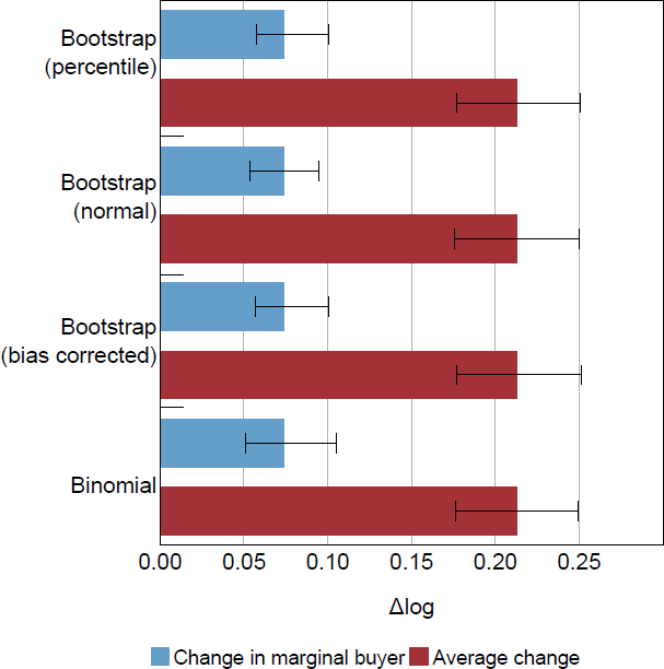
B.1.1 Binomial method of confidence intervals
Denote the true underlying CDFs of the WTPs with a 20 per cent down payment F20(x). The first stage of the procedure is to estimate the percentile F20(0), noting that zero is the log of the ratio of relative WTP equal to the appraisal. The binomial confidence interval procedure works using the logic that whether or not a given WTP is higher than this level has probability F20(0). A binomial distribution with success probability F20(0) and the number of trials given by the number of WTPs can then map out a confidence interval for the estimate of the percentile (0). A similar method can be used for the second stage to construct a confidence interval for the WTP at the estimated percentile of the other demand curve, and the two are combined for the overall confidence interval.
In more detail:
The object of interest for the first stage in the marginal buyer procedure is the value of the underlying CDF at F20(0). I will call the point estimate The goal is to get a lower and upper bound (pL and pU) consistent with a level of significance .
To construct the lower bound of the confidence interval, I find the smallest pL such that is not rejected. Let S equal the number of WTPs < 0 and n equal the total sample size of WTPs. Under the null, S is the test statistic, and it follows a binomial distribution based on the success probability pL and sample size n, i.e. S ~ B(n, pL). The null is rejected if the CDF of the binomial is less than the level of significance: BCDF(S, (n, pL)) < . So for the lower bound this binds with equality.
Similarly the upper bound is given by ( 1 – BCDF(S, (m, pU)) ) = .
The second stage of the procedure is a similar process in reverse. For the purposes of this stage I will take the estimate from the first stage as a true parameter, p. The goal is then to estimate the upper and lower bounds on the WTP given by . The point estimate for this is .
Now the relevant null hypothesis for the lower bound is H0 : WTPL = . We know the relevant binomial distribution has success probability p and sample size n. To test H0 count the WTPs < WTPL, and call that number T. Then reject if BCDF (T, (n, p)) The lower bound is given by WTPL that corresponds to the T where this holds with equality.
Similarly, the upper bound is given by the Tth WTP where (1 – BCDF(T, (n, p))) =
To combine the two steps into a confidence interval of size for the whole process I construct a confidence interval for the first stage using a level of significance of . I then do the second stage on the upper and lower bounds of that confidence interval again with level of significance The resulting lower confidence bound from the lower input percentile and upper confidence bound from the upper input percentile form the appropriate confidence interval.
There is substantial skew in the data, with a median change of zero. The range of average changes over different trim depths is very large and it is hard to recommend one in particular. The change in WTP of the marginal buyer is much less sensitive to the trim depth, being pretty consistent from no trimming up to a 30 per cent trim (see Figures B2–B4).
Note:
Dashed lines represent 95 per cent confidence intervals.
Note:
Dashed lines represent 95 per cent confidence intervals.
Note:
Dashed lines represent 95 per cent confidence intervals.
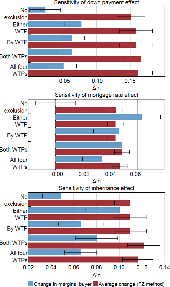
A WTP equal to the appraisal value creates a flat demand curve, which makes it hard to interpret changes (Figure B5). For robustness, I try five different exclusion methods for each of the three experimental conditions, which I explain below.
The five methods I use in order from least exclusion to most exclusion are as follows. If there is still a flat area of the demand curve after exclusion, I assume the supply curve is in the middle of it.
Figure B6 shows the results of the five different methods. The results of the down payment experiment are insensitive to the exclusion method. Small changes to the demand curve and the marginal buyer do not change the overall picture. For all methods, the marginal buyer method is significantly less than the mean change, and there are no significant differences between the estimates of each effect by the five methods. In contrast, the results of the mortgage rate do vary significantly depending on the exclusion method. The lack of systematic relationship between the shift size and the position on the demand curve means small changes can have noticeable effects on the marginal buyer. The sensitivity of the inheritance experiment is somewhere in between.
Note:
Whiskers show 95 per cent confidence intervals.
B.2 How much to trim?
B.3 Sensitivity of the results to treatment of WTPs equal to appraisal
Appendix C: Modelling
C.1 Preference parameters and the nonlinear mapping
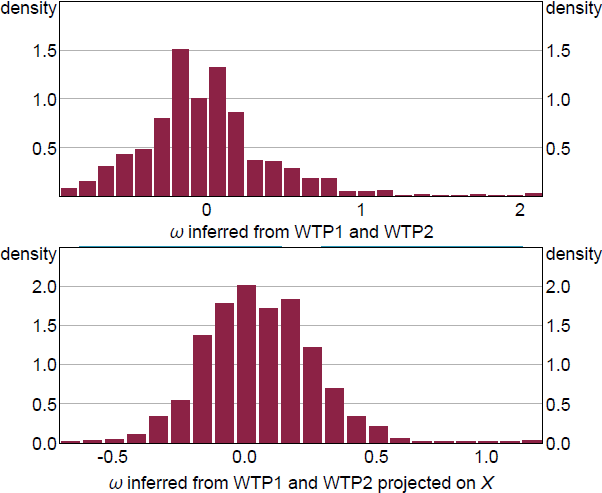
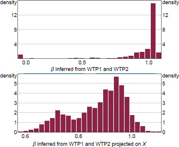
The fitted distributions are narrower than the distributions inferred from the WTP data. The fitted distribution can be thought of as the heterogeneity that can be accounted for by the observable financial and demographic data, while the inferred distribution captures all heterogeneity in responses. The rent/own preference parameter distribution is reasonably well captured in the fitted distribution. The heterogeneity of the time preference parameter that governs the increase in WTP is not well captured by observable variables. Idiosyncratic heterogeneity is clearly important. There are two modes in the actual distribution but none of the explanatory variables capture this feature of the distribution.
C.2 User cost prediction equations
where the and coefficients are estimated in regressions
The willingness to pay in each condition (WTP20 and WTP5) are then found by plugging and into the heterogeneous user cost equation (Equation (2)) with the two values of the down payment constraint, .
Appendix D: Estimation Results for Full Set of Explanatory Variables
| WTP20% | ||||
|---|---|---|---|---|
| Interest rate low | −0.01 | 0.03* | −0.04 | −0.29*** |
| Owner | −0.14** | 0.10*** | 0.14 | −0.00 |
| Age | −0.00** | 0.00** | 0.00 | −0.00** |
| Total numeracy | −0.01 | 0.00 | 0.03 | −0.04 |
| College | 0.00 | 0.00 | −0.02 | −0.04 |
| Male | 0.01 | −0.01 | 0.10 | 0.13** |
| Marginal income tax rate | 0.00 | −0.00 | 0.00 | 0.01 |
| Property tax rate | 0.07*** | −0.04*** | −0.01 | 0.16*** |
| Risk averse | 0.00 | 0.00 | −0.05 | −0.00 |
| Risk loving | −0.01 | 0.01 | 0.04 | 0.11 |
| E(inc growth, 1 yr) | −0.00 | −0.00 | −0.00 | −0.00 |
| E(HP growth, 1 yr) | −0.00* | 0.00 | −0.00 | −0.01** |
| Pr(move over next 3 yrs) | 0.00 | −0.00 | 0.00 | 0.00 |
| Pr(buy|move) | 0.00 | −0.00 | 0.01*** | 0.00*** |
| Equity in (0, 50K] | −0.09 | 0.05 | 0.44*** | 0.05 |
| Equity in (50K, 125K] | −0.13** | 0.07* | 0.49*** | −0.10 |
| Equity in (125K, 200K] | −0.10 | 0.05 | 0.37** | −0.15 |
| Equity of more than 200K | −0.13** | 0.07 | 0.31* | −0.25* |
| Liquid savings of [5K, 30K) | 0.02 | −0.02 | 0.12 | −0.00 |
| Liquid savings of [30K, 100K) | −0.07* | 0.04* | 0.22** | 0.05 |
| Liquid savings of [100K, 500K) | −0.04 | 0.02 | 0.12 | 0.13 |
| Liquid savings of 500K or more | −0.01 | 0.01 | 0.35** | 0.26** |
| Non-housing debt of [1K, 5K) | −0.01 | 0.00 | −0.14 | −0.11 |
| Non-housing debt of [5K, 30K) | 0.01 | −0.01 | −0.02 | −0.10 |
| Non-housing debt of 30K or more | 0.01 | −0.01 | −0.16* | −0.14* |
| Credit score 680–719 | −0.06 | 0.04 | 0.08 | −0.15 |
| Credit score 720–760 | −0.08** | 0.05* | 0.18 | −0.11 |
| Credit score above 760 | −0.08** | 0.05** | 0.13 | −0.12 |
| Income in (40K, 75K] | −0.02 | 0.01 | −0.06 | −0.04 |
| Income in (75K, 150K] | −0.05 | 0.04 | −0.01 | −0.03 |
| Income greater than 150K | −0.10* | 0.07* | −0.05 | −0.17 |
| Constant | 0.36*** | 0.75*** | −1.50*** | 0.33 |
| Observations | 789 | 789 | 789 | 754 |
| R2 | 0.217 | 0.212 | 0.227 | 0.179 |
| RMSE | 0.30 | 0.20 | 0.87 | 0.68 |
|
Note: ***, ** and * denote statistical significance at the 1, 5 and 10 per cent levels, respectively. Sources: Author's calculations; Fuster and Zafar (2021) |
||||
Appendix E: Data Sources
The dataset from Fuster and Zafar (2021) is available with the publication at <https://doi.org/10.1257/pol.20150337>. The other household datasets are sourced from national bodies.
US Survey of Consumer Finances is from the Federal Reserve Board at <https://www.federalreserve.gov/econres/scfindex.htm>.
The Australian Survey of Income and Housing is from the Australian Bureau of Statistics (access permission required) at <https://www.abs.gov.au/statistics/microdata-tablebuilder/available-microdata-tablebuilder/income-and-housing-australia>.
The Swiss Household Panel is from The FORS Centre (access permission required) at <https://forscenter.ch/projects/swiss-household-panel/>.
Bank of Spain Survey of Household Finances is from NORC at the University of Chicago (access permission required) at <https://www.norc.org/Research/Projects/Pages/bank-of-spain-survey-of-household-finances.aspx>.
References
Acharya VV, K Bergant, M Crosignani, T Eisert and F McCann (2020), ‘The Anatomy of the Transmission of Macroprudential Policies’, IMF Working Paper No WP/20/58.
Adelino M, A Schoar and F Severino (2016), ‘Loan Originations and Defaults in the Mortgage Crisis: The Role of the Middle Class’, The Review of Financial Studies, 29(7), pp 1635–1670.
Albanesi S, G De Giorgi and J Nosal (2017), ‘Credit Growth and the Financial Crisis: A New Narrative’, NBER Working Paper No 23740.
Alvarez FE and DO Argente (2020), ‘Consumer Surplus of Alternative Payment Methods: Paying Uber with Cash’, NBER Working Paper No 28133.
Armstrong J, H Skilling and F Yao (2019), ‘Loan-to-Value Ratio Restrictions and House Prices: Micro Evidence from New Zealand’, Journal of Housing Economics, 44, pp 88–98.
Bellemare MF and CJ Wichman (2020), ‘Elasticities and the Inverse Hyperbolic Sine Transformation’, Oxford Bulletin of Economics and Statistics, 82(1), pp 50–61.
Ben-David I, P Towbin and S Weber (2019), ‘Expectations during the U.S. Housing Boom: Inferring Beliefs from Actions’, NBER Working Paper No 25702, March.
Colwell P and J Trefzger (2005), ‘Supply-Side Effects and Contingent Valuation Analysis’, Journal of Real Estate Practice and Education, 8(1), pp 45–59.
Corbae D and E Quintin (2015), ‘Leverage and the Foreclosure Crisis’,Journal of Political Economy, 123(1), pp 1–65.
Cox J and SC Ludvigson (2021), ‘Drivers of the Great Housing Boom-Bust: Credit Conditions, Beliefs, or Both?’, Real Estate Economics, 49(3), pp 843–875.
Cusbert T (2022), ‘Credit Supply and the Housing Boom: The Role of Renters and Landlords’, in Essays on Asset Pricing in Incomplete Markets, PhD thesis, The University of Sydney, pp 34–67.
Duca JV, J Muellbauer and A Murphy (2021), ‘What Drives House Price Cycles? International Experience and Policy Issues’, Journal of Economic Literature, 59(3), pp 773–864.
Favilukis J, SC Ludvigson and S Van Nieuwerburgh (2017), ‘The Macroeconomic Effects of Housing Wealth, Housing Finance, and Limited Risk Sharing in General Equilibrium’, Journal of Political Economy, 125(1), pp 140–223.
Foote CL, L Loewenstein and PS Willen (2016), ‘Cross-Sectional Patterns of Mortgage Debt during the Housing Boom: Evidence and Implications’, NBER Working Paper No 22985.
Fuster A and B Zafar (2021), ‘The Sensitivity of Housing Demand to Financing Conditions: Evidence from a Survey’, American Economic Journal: Economic Policy, 13(1), pp 231–265.
Garriga C, R Manuelli and A Peralta-Alva (2019), ‘A Macroeconomic Model of Price Swings in the Housing Market’, The American Economic Review, 109(6), pp 2036–2072.
Glaeser EL, JD Gottlieb and J Gyourko (2012), ‘Can Cheap Credit Explain the Housing Boom?’, in EL Glaeser and T Sinai (eds), Housing and the Financial Crisis, National Bureau of Economic Research Conference Report, University of Chicago Press, Chicago, pp 301–359.
Graham J (2020), ‘House Prices, Investors, and Credit in the Great Housing Bust’, Job Market Paper, New York University, 25 November.
Greenwald DL and A Guren (2021), ‘Do Credit Conditions Move House Prices?’, NBER Working Paper No 29391.
Iacoviello M (2005), ‘House Prices, Borrowing Constraints, and Monetary Policy in the Business Cycle’, The American Economic Review, 95(3), pp 739–764.
Justiniano A, GE Primiceri and A Tambalotti (2019), ‘Credit Supply and the Housing Boom’, Journal of Political Economy, 127(3), pp 1317–1350.
Kaplan G, K Mitman and GL Violante (2020), ‘The Housing Boom and Bust: Model Meets Evidence’, Journal of Political Economy, 128(9), pp 3285–3345.
La Cava G and L Wang (2021), ‘The Rise in Household Liquidity’, RBA Research Discussion Paper No 2021-10.
Landvoigt T, M Piazzesi and M Schneider (2015), ‘The Housing Market(s) of San Diego’, The American Economic Review, 105(4), pp 1371–1407.
Mian A and A Sufi (2009), ‘The Consequences of Mortgage Credit Expansion: Evidence from the U.S. Mortgage Default Crisis’, The Quarterly Journal of Economics, 124(4), pp 1449–1496.
Mian A and A Sufi (2017), ‘Fraudulent Income Overstatement on Mortgage Applications during the Credit Expansion of 2002 to 2005’, The Review of Financial Studies, 30(6), pp 1832–1864.
Richter B, M Schularick and I Shim (2019), ‘The Costs of Macroprudential Policy’, Journal of International Economics, 118, pp 263–282.
Van Bekkum S, M Gabarro, RM Irani and JL Peydró (2019), ‘Take It to the Limit? The Effects of Household Leverage Caps’, Centre for Economic Policy Research Discussion Paper No DP13503, rev 15 June 2020.
Acknowledgements
An earlier draft of this paper formed part of my PhD dissertation at the University of Sydney. Many thanks to Andreas Fuster and Basit Zafar for sharing their data before its public release, and to my primary adviser Chris Gibbs. I have also benefited from useful comments and feedback from James Morley, Andreas Fuster, Greg Kaplan, Aarti Singh, Alex Ballantyne, Anirudh Yadav, Sarah Quincy, Gianni La Cava, Anthony Brassil, Simon (Yunho) Cho, Ivan Roberts, John Simon, Luci Ellis, and participants of the University of Sydney HDR Workshop, Sydney MRG Workshop 2020, and the North American Urban Economics Association Meetings 2021. The views expressed in this paper are those of the author and should not be attributed to the Reserve Bank of Australia. Any errors are the sole responsibility of the author.
Footnotes
If the respondent owns their current home, the question states that they sell it and discharge their mortgage before making the down payment on their new hypothetical home. [1]
The only example of a similar method I am aware of is in a real estate valuation paper that estimates the price effect of negative amenities like high-voltage power lines or environmental contamination (Colwell and Trefzger 2005). [2]
See the online appendix, available at <https://doi.org/10.1257/pol.20150337>. [3]
Colwell and Trefzger (2005) also assume a vertical supply curve in their demand curve analysis in the context of modelling the price effect of a disamenity. [4]
A substantial fraction of respondents give a WTP exactly equal to the home value. This may be related to differing interpretations of the question, and makes the interpretation of the curves difficult. For my main results I remove any WTP equal to the home value to eliminate the flat spot in the demand curve. Appendix B.3 shows that the down payment results are not sensitive to this treatment. [5]
Appendix B.1 shows that the confidence intervals are similar for a range of different bootstrap methods as well as a non-parametric binomial method. [6]
In the United States, mortgage interest is tax deductible up to a limit. [7]
I solve for the preference parameters using WTPs from first two questions (i.e. just using the two down payment conditions). Results are similar if I include the third question with a different interest rate and fit the two preference parameters by maximum likelihood. I do not consider the inheritance condition because it does not map as well to the user cost model. [8]
Appendix C.1 shows the distribution of each parameter individually. [9]
Details of these full regressions are in Appendix C.2. [10]
Using the inverse hyperbolic sine transformation means the coefficient and marginal effect estimates depend on the scale of the variable, with it closely approximating a log transformation above 10 (see Bellemare and Wichman (2020)). I include the available equity as a percentage, that is . Including it as a fraction makes it close to linear because the magnitudes are frequently close to zero and often less than 1. It also degrades the fit of the model. [11]
Take, for example, the bottom end of the demand curves in Michigan (see Figure 1) and Illinois. Both show large responses to the down payment change, but the 20 per cent WTP in Illinois looks a bit like the respondent accidentally wrote US$10,000 instead of US$100,000 given they have US$5,000 in home equity and US$7,500 in liquid savings. Whereas the low response in the Michigan demand curve is more consistent with their zero liquid savings. But this is guess work. [12]
It is rare for surveys to include an estimate of the home value of renters, so I use actual rent paid together with data on rental yields. [13]
The SIH is a biennial household survey that collects information on income, wealth, housing and various other household and personal characteristics. I omit the 2007/08 SIH as some of the wealth variables were not collected. [14]
The simulated demand curves for each year look very similar to the simulation for US data in Figures 10 and 11. [15]