RDP 2022-04: The Unit-effect Normalisation in Set-identified Structural Vector Autoregressions 5. The Effects of a 100 Basis Point Federal Funds Rate Shock
October 2022
- Download the Paper 2,225KB
This section illustrates the empirical relevance of the issues discussed above by estimating the macroeconomic effects of a 100 basis point shock to the federal funds rate under different sets of identifying restrictions that have been used in the literature.
I use the reduced-form VAR considered in Uhlig (2005), Antolín-Díaz and Rubio-Ramírez (2018) and Arias et al (2019). The model's endogenous variables are real GDP (GDPt), the GDP deflator (GDPDEFt), a commodity price index (COMt), total reserves (TRt), non-borrowed reserves (NBRt) (all in natural logarithms) and the federal funds rate (FFRt). I order the variables such that yt = (FFRt, GDPt, GDPDEFt, COMt, TRt, NBRt)', so is the impact response of the federal funds rate to a monetary policy shock. The data are monthly and run from January 1965 to November 2007.[17] The VAR includes 12 lags of the variables and a constant. I assume a Jeffreys' prior over the reduced-form parameters, so This means that the posterior for is a normal-inverse-Wishart distribution, from which it is straightforward to obtain independent draws (e.g. Del Negro and Schorfheide 2011).
The papers listed above conduct Bayesian inference under a uniform prior for Q and primarily present impulse responses to a standard deviation monetary policy shock.[18] In contrast, I focus on the impulse responses to a 100 basis point monetary policy shock and assess the sensitivity of posterior inferences to the choice of prior by conducting robust Bayesian inference. Appendix C describes the numerical algorithms used to implement the inferential procedures applied in this section.
First, I consider the identifying restrictions proposed in Arias et al (2019), who impose sign and zero restrictions on the structural equation for the federal funds rate, which they interpret as a monetary policy reaction function. The restrictions impose that the coefficients on TRt and NBRt in the structural equation for FFRt are zero, which means that the Federal Reserve does not react to changes in reserves when setting the federal funds rate. They also impose sign restrictions on the coefficients of GDPt and GDPDEFt such that the Federal Reserve does not increase the federal funds rate in response to lower output or prices, which is consistent with the types of policy rules typically specified in New Keynesian dynamic stochastic general equilibrium (DSGE) models. The impact response of FFRt to the monetary policy shock is restricted to be non-negative, so that a monetary policy shock does not decrease FFRt on impact, which seems natural. I denote this set of identifying restrictions as Restriction (1).
Figure 3 presents the impulse responses of FFRt and GDPt to a 100 basis point monetary policy shock obtained under Restriction (1) and a conditionally uniform prior for Q . The 68 per cent (equi-tailed) credible intervals include declines in output of close to 4 per cent and the 90 per cent confidence intervals include declines in output exceeding 10 per cent, so there is considerable posterior probability assigned to very large declines in output.
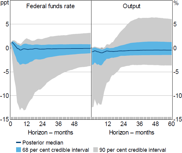
Note: Results obtained under the identifying restrictions in Arias et al (2019); based on 10,000 draws from the posterior of the reduced-form parameters.
The very wide credible intervals suggest that the identifying restrictions are quite uninformative about the output response to a 100 basis point monetary policy shock. However, even these very wide credible intervals severely overstate the informativeness of the restrictions. The restrictions include four sign restrictions (including the sign normalisation on the (1,1) element of A0) and two zero restrictions, so the total number of restrictions is equal to the number of variables in the VAR. This means that the sufficient condition in Proposition 4.2 is satisfied, and zero is always included within the identified set for the impact response of the federal funds rate; in other words, the identifying restrictions cannot rule out the possibility that the federal funds rate does not respond to a standard deviation monetary policy shock on impact. In turn, this suggests that identified sets for unit impulse responses have the potential to be unbounded for all draws of . Examining the approximated bounds of the identified sets for the output responses to a 100 basis point shock suggests that these identified sets are indeed unbounded at every draw, which in turn suggests that the robust credible intervals are unbounded at all credibility levels.[19] The shape of the posterior distribution under the standard approach to inference therefore appears to be driven entirely by the conditional prior.
Next, I combine the restrictions from Arias et al (2019) with the sign restrictions on impulse responses proposed in Uhlig (2005). These sign restrictions impose that the impulse response of FFRt+h to the monetary policy shock is non-negative and the impulse responses of GDPDEFt+h, COMt+h and NBRt+h are non-positive for h = 0,1,..,5.[20] I refer to this set of restrictions as Restriction (2). Under a conditionally uniform prior, the additional sign restrictions appreciably tighten the posterior distribution of the impulse responses to a 100 basis point shock (Figure 4). The posterior median suggests that output falls by a maximum of around 0.4 per cent about two years after the shock and the 68 per cent credible intervals no longer contain extremely large output responses; for example, at the two-year horizon the credible intervals span declines in output of 0.1-0.6 per cent. However, I discuss below that these results are highly sensitive to the choice of conditional prior.
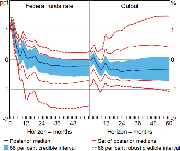
Note: Results obtained under a combination of the identifying restrictions in Uhlig (2005) and Arias et al (2019); based on 10,000 draws from the posterior of the reduced-form parameters.
Under these restrictions, there are 2 zero restrictions and 27 sign restrictions, so the sufficient condition in Proposition 4.2 is not satisfied. This means that the identified set for the impact response of the federal funds rate does not necessarily include zero. I therefore numerically check whether the identified set for includes zero at each draw from the reduced-form posterior. The identified set for includes zero in only 0.06 per cent of draws from the posterior, which implies that the identified sets for the impulse responses to a 100 basis point shock are guaranteed to be bounded with very high posterior probability. It follows that the set of posterior medians is guaranteed to be bounded, as are robust credible intervals at conventional credibility levels (see Remark 4.1). However, the set of posterior medians for the output response includes zero at essentially all horizons, and the 68 per cent robust credible intervals for the output response include both large negative and large positive responses. Hence, the data and identifying restrictions are consistent with either relatively large decreases or increases in output following a 100 basis point shock, and the identifying restrictions are reasonably uninformative about the output response.
These results indicate that much of the apparent information in the standard Bayesian posterior under Restriction (2) is contributed by the conditional prior rather than the data and identifying restrictions, and posterior inferences are sensitive to the choice of conditional prior. To quantify the information contributed by the conditional prior, Giacomini and Kitagawa (2021) suggest reporting the ‘prior informativeness’ statistic; this measures the fraction that the credible interval is tightened (relative to the robust credible interval) by choosing a particular conditional prior. The prior informativeness statistic for the output response is around 70 per cent for the horizons considered (i.e. the 68 per cent credible intervals are around 30 per cent as wide as the 68 per cent robust credible intervals).
Finally, I add the ‘narrative restrictions’ proposed in Antolín-Díaz and Rubio-Ramírez (2018) to Restriction (2). I refer to this set of restrictions as Restriction (3). Narrative restrictions are restrictions on functions of the structural shocks in specific periods (as opposed to restrictions on functions of the structural parameters) that represent information about the nature of the shocks hitting the economy during particular historical episodes.[21] The specific narrative restrictions imposed are that the monetary policy shock was positive and was the ‘overwhelming’ contributor to the forecast error in the federal funds rate in October 1979. This is the month in which the Federal Reserve unexpectedly and dramatically raised the federal funds rate following Paul Volcker becoming chairman, and is widely considered an example of a monetary policy shock (e.g. Romer and Romer 1989).
Under Restriction (3), the identified set for the impact response of the federal funds rate excludes zero in 100 per cent of draws from the reduced-form posterior. Consequently, the set of posterior medians and the robust credible intervals are bounded at all credibility levels. The set of posterior medians for the output response excludes zero at most horizons and the 68 per cent robust credible intervals are substantially narrower than under Restriction (2) (Figure 5). Nevertheless, the robust credible intervals continue to include zero at all horizons and the choice of conditional prior contributes a large share of the information contained in the posterior; the prior informativeness statistic for the output response ranges from around 70 per cent at shorter horizons to around 50 per cent at longer horizons.
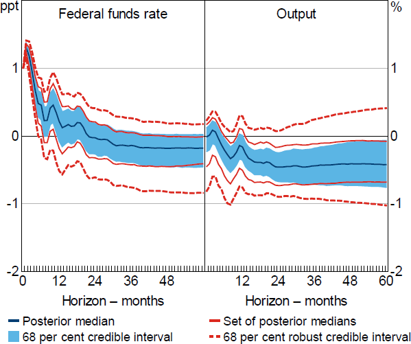
Note: Results obtained under a combination of the identifying restrictions in Uhlig (2005), Antolín-Díaz and Rubio-Ramírez (2018) and Arias et al (2019); based on 1,000 draws from the posterior of the reduced-form parameters.
Table 1 tabulates the posterior lower and upper probabilities that output falls by more than a given threshold x at selected horizons. Under Restriction (2), the posterior lower and upper probabilities that the output response is negative include both small values and values close to one at all horizons, which indicates that the data and identifying restrictions are fairly uninformative about the sign of the output response. In contrast, under Restriction (3), the posterior lower probability that the output response is negative at the two-year horizon is around 75 per cent and the posterior upper probability is 100 per cent. The hypothesis that output declines following a 100 basis point monetary policy shock therefore receives reasonably high posterior probability uniformly over the class of posteriors that are consistent with Restriction (3). Both sets of identifying restrictions effectively rule out relatively large declines in output following a 100 basis point shock; for example, under Restriction (3), the posterior lower probability that output declines by more than 1 per cent two years after the shock is zero and the posterior upper probability is only 6 per cent.
The existing literature contains a wide range of estimates for the output effects of a 100 basis point shock to the federal funds rate; for example, Ramey (2016) reports a range of existing estimates for the trough in the response of output under different samples, specifications and approaches to identification. These estimates range from as low as 0.6 per cent to as high as 5 per cent. The results in Table 1 are broadly consistent with the output effects of monetary policy lying towards the smaller end of the range of existing estimates, in the sense that relatively large output declines are assigned low posterior probability regardless of the choice of conditional prior.
| Horizon | Threshold | ||||||||
|---|---|---|---|---|---|---|---|---|---|
| Lower probability (%) | Upper probability (%) | ||||||||
| 0 | −0.25 | −0.5 | −1 | 0 | −0.25 | −0.5 | −1 | ||
| Restriction (2) | |||||||||
| Impact | 0.00 | 0.00 | 0.00 | 0.00 | 0.95 | 0.75 | 0.48 | 0.10 | |
| One year | 0.13 | 0.01 | 0.00 | 0.00 | 0.99 | 0.84 | 0.48 | 0.06 | |
| Two years | 0.27 | 0.11 | 0.03 | 0.00 | 1.00 | 1.00 | 0.93 | 0.07 | |
| Three years | 0.23 | 0.11 | 0.04 | 0.00 | 1.00 | 0.99 | 0.88 | 0.11 | |
| Four years | 0.23 | 0.12 | 0.05 | 0.00 | 1.00 | 0.98 | 0.80 | 0.15 | |
| Restriction (3) | |||||||||
| Impact | 0.00 | 0.00 | 0.00 | 0.00 | 0.95 | 0.73 | 0.45 | 0.04 | |
| One year | 0.27 | 0.03 | 0.00 | 0.00 | 0.99 | 0.84 | 0.47 | 0.04 | |
| Two years | 0.76 | 0.36 | 0.08 | 0.00 | 1.00 | 1.00 | 0.93 | 0.06 | |
| Three years | 0.64 | 0.33 | 0.11 | 0.01 | 1.00 | 0.99 | 0.88 | 0.10 | |
| Four years | 0.57 | 0.30 | 0.12 | 0.01 | 1.00 | 0.98 | 0.79 | 0.13 | |
| Note: Posterior lower (upper) probability is the smallest (largest) posterior probability obtainable within the class of posteriors consistent with the identifying restrictions. | |||||||||
Footnotes
I use the dataset from Antolín-Díaz and Rubio-Ramírez (2018). The monthly series for GDPt and GDPDEFt are obtained by interpolation; see Arias et al (2019) for details. [17]
Uhlig (2005) and Arias et al (2019) present impulse responses to a standard deviation shock. Antolín-Díaz and Rubio-Ramírez (2018) present impulse responses that are normalised such that the median impact response of the federal funds rate is 25 basis points; this differs to the unit-effect normalisation, where the impact response of the federal funds rate is normalised at every draw from the posterior. [18]
For example, the minimum width of the identified set for the impact response of output across the posterior draws is on the order of 100 percentage points and the maximum width is on the order of 108 percentage points. [19]
Uhlig (2005) also considers restricting the impulse responses at shorter and longer horizons than six months. The choice of horizon here does not affect whether the sufficient condition in Proposition 4.2 applies. However, the proportion of draws where the identified set for includes zero varies across the different sets of restrictions, as does the width of the sets of posterior medians and robust credible intervals. Appendix D presents the output responses obtained when the impulse responses are restricted up to horizon [20]
The narrative restrictions are functions of the data through the reduced-form VAR innovations that enter the restrictions (i.e. they do not only depend on ). Consequently, the standard definition of an identified set does not apply; Giacomini, Kitagawa and Read (2021a) instead introduce the concept of a ‘conditional’ identified set, which is the identified set that would be obtained after conditioning on the data that directly enter the narrative restrictions. I refer to the identified set interchangeably with the conditional identified set. [21]