Research Discussion Paper – RDP 2022-04 The Unit-effect Normalisation in Set-identified Structural Vector Autoregressions
1. Introduction
Estimating the response of the economy to macroeconomic shocks (such as monetary policy shocks) is difficult, because it requires disentangling the effects of the shock from the effects of other shocks hitting the economy at the same time. Macroeconomists do this by imposing ‘identifying restrictions’, which are assumptions about the structure of the economy. When using structural vector autoregression (SVAR) models, researchers have traditionally imposed identifying restrictions that are sufficient to pin down the responses to the shocks of interest, in which case we say that the responses are ‘point identified’. However, it has become increasingly common to impose arguably weaker sets of identifying restrictions at the expense of only being able to determine a set of possible responses, in which case we say that the effects are ‘set identified’. These weaker sets of restrictions often take the form of restrictions on the signs of impulse responses to shocks (e.g. Uhlig 2005).
Set-identified SVARs are typically estimated under the normalisation that structural shocks have unit standard deviation. The impulse responses that are obtained under this ‘standard deviation normalisation’ consequently represent impulse responses to a standard deviation shock. However, these impulse responses often do not answer the pertinent economic question. For instance, central bankers are interested in answering questions like ‘what are the effects of a 100 basis point increase in the policy rate?’ To answer this question, we need to know what happens following a monetary policy shock that results in a 100 basis point increase in the policy rate. The responses to a ‘unit shock’ – a shock that raises a particular variable by one unit – are therefore naturally more relevant in this setting (and many others). Such responses can be obtained under the ‘unit-effect normalisation’ (Fry and Pagan 2011; Stock and Watson 2016, 2018). In this paper, I explore the extent to which set-identifying restrictions are informative about impulse responses to unit shocks (or ‘unit impulse responses’).
Set-identifying restrictions generate an ‘identified set’ for the impulse responses, which is the set of impulse responses that are consistent with the data given the identifying restrictions. The identified set for a unit impulse response may be unbounded (Baumeister and Hamilton 2015, 2018). This implies that set-identifying restrictions may be extremely uninformative about the effects of a unit shock, which is a point that appears to have been underappreciated in the literature.[1] A contribution of this paper is to highlight this issue and explain why it arises.
To provide some intuition about why the identified set for a unit impulse response may be unbounded, consider estimating the response of output to a monetary policy shock. The impulse response of output to a 100 basis point monetary policy shock can be defined as the impulse response of output divided by the impact response of the policy rate (the ‘normalising impulse response’), where both impulse responses are with respect to a standard deviation monetary policy shock. The identifying restrictions may admit the possibility that the policy rate does not respond on impact to the shock; in other words, the identified set for the normalising impulse response may include zero. In this case, it may be possible to make the impulse response of output to a 100 basis point shock arbitrarily large in magnitude by considering a sequence of parameters converging to the point where the impact response of the policy rate is zero.[2]
I discuss how researchers can draw useful inferences about unit impulse responses when the identified set is potentially unbounded, with a focus on the prior robust approach to Bayesian inference proposed in Giacomini and Kitagawa (2021). As elaborated on below, this is a natural approach to conducting Bayesian inference in set-identified models, because it eliminates the problem of posterior sensitivity to the choice of prior that arises in this setting. Section 2 describes the modelling framework and outlines the robust Bayesian approach to inference. The key feature of this approach to inference is that it replaces the prior distribution with a class of priors, which contains all priors that are consistent with the identifying restrictions. In turn, the class of priors generates a class of posteriors. Summarising the class of posteriors requires computing the lower and upper bounds of the identified set for each impulse response. Importantly, whether different summaries of the class of posteriors are bounded will depend on the posterior probability that the identified set is bounded. I therefore argue that it is crucial to understand how often the identified set is unbounded in any given application, since this helps to communicate transparently about the informativeness of the identifying restrictions.
To make these issues clear, I use a bivariate SVAR in which I can analytically characterise identified sets under some sign restrictions on impulse responses (Section 3). I then explain how to verify whether identified sets for the impulse responses to a unit shock may be unbounded in an SVAR of arbitrary dimension identified using both sign and zero restrictions (Section 4). I show that a necessary condition for unboundedness of these identified sets is that zero is included within the identified set for the normalising impulse response. I then provide an easily verifiable sufficient condition under which the identified set for the normalising impulse response includes zero; specifically, if the number of sign and zero restrictions is no greater than the number of variables in the SVAR and the restrictions relate to a single structural shock, the identified set for the normalising impulse response always includes zero. When this sufficient condition is not satisfied (i.e. when there are more restrictions than variables in the SVAR and/or the restrictions relate to multiple shocks), the identified set for the normalising impulse response may or may not include zero. In this case, I explain how to numerically check whether the identified set for the normalising impulse response includes zero. Ultimately, I recommend that researchers report the posterior probability that the normalising impulse response includes zero, since this makes it clear which summaries of the class of posteriors are guaranteed to be bounded.
To illustrate the importance of these issues in practice, I estimate the macroeconomic effects of a 100 basis point shock to the federal funds rate under different combinations of identifying restrictions (Section 5): the sign restrictions on impulse responses to a monetary policy shock proposed in Uhlig (2005); the sign and zero restrictions on the systematic component of monetary policy proposed in Arias, Caldara and Rubio-Ramírez (2019); and the ‘narrative restrictions’ proposed in Antolín-Díaz and Rubio-Ramírez (2018).
Under the restrictions considered in Arias et al (2019), the sufficient condition described above is satisfied, so zero is always included in the identified set for the normalising impulse response; that is, the identifying restrictions never rule out models in which the federal funds rate does not respond on impact to a monetary policy shock. This indicates that identified sets for the impulse responses to a 100 basis point shock may always be unbounded. Numerical approximations of the bounds of the identified set suggest that this is indeed the case. These restrictions are therefore extremely uninformative about the effects of a 100 basis point shock.
Combining the restrictions from Arias et al (2019) with the sign restrictions on impulse responses considered in Uhlig (2005) yields identified sets that are bounded with posterior probability close to, but less than, 100 per cent. Nevertheless, the class of posteriors is consistent with either relatively large decreases or increases in output following a 100 basis point shock, so the identifying restrictions appear to be fairly uninformative about the output response to the shock.
Additionally imposing narrative restrictions on the monetary policy shock (as in Antolín-Díaz and Rubio-Ramírez (2018)) yields identified sets that are bounded at every posterior draw of the reduced-form parameters. The results under this set of restrictions are consistent with the peak effects of monetary policy on output lying towards the smaller end of the range of existing estimates summarised in Ramey (2016).
Finally, I discuss the possibility of using alternative identifying restrictions to ensure that identified sets for unit impulse responses are bounded (Section 6). For instance, I consider directly bounding the normalising impulse response away from zero. However, I argue that it may be difficult to elicit a credible lower bound and inferences may be sensitive to changes in the imposed bound. I conclude that such restrictions are unlikely to be a satisfactory solution.
1.1 Related literature
An extensive literature uses set-identified SVARs to estimate the effects of macroeconomic shocks.[3] Under the standard approach to Bayesian inference in set-identified SVARs (e.g. Uhlig 2005; Rubio-Ramírez, Waggoner and Zha 2010; Arias, Rubio-Ramírez and Waggoner 2018), it is straightforward to transform from the standard deviation normalisation to the unit-effect normalisation; this transformation simply requires dividing the impulse responses obtained under the standard deviation normalisation by the normalising impulse response.[4] Repeating this at each draw of the parameters from their posterior distribution generates a posterior distribution for the impulse responses to a unit shock. However, there are well-documented problems with the standard approach to Bayesian inference in set-identified models. In particular, because the model is set identified, the likelihood function is flat with respect to certain parameters. As a consequence, a component of the prior is ‘unrevisable’ in the sense that it is never updated, and posterior inference may be sensitive to the choice of prior (e.g. Poirier 1998).[5]
Baumeister and Hamilton (2015) show that the ‘uniform’ prior that is used in the standard approach to Bayesian inference does not necessarily induce a uniform prior over the parameters that are typically of interest, such as impulse responses. They argue that this prior may therefore drive posterior inference despite not reflecting the researcher's actual prior beliefs. As an alternative, they suggest that researchers should impose a prior directly over the structural parameters (see also Baumeister and Hamilton (2018, 2019)). It remains the case under this approach that a component of the prior will never be updated, so posterior sensitivity to the choice of prior may still be a concern.
To address the problem of posterior sensitivity in set-identified models, Giacomini and Kitagawa (2021) propose conducting Bayesian inference using an approach that is robust to the choice for the unrevisable component of the prior. When applying this approach in a set-identified SVAR, they focus on the impulse responses to standard deviation shocks as the parameters of interest. Giacomini, Kitagawa and Read (2022b) describe an algorithm for conducting robust Bayesian inference in proxy SVARs (i.e. SVARs identified using an external instrument) under the unit-effect normalisation. They note that the identified set may be unbounded, but do not draw out the implications of this issue for conducting inference. Baumeister and Hamilton (2015, 2018) explicitly show that the identified set may be unbounded in a simple bivariate model identified with sign restrictions. My own bivariate example builds on their setting by: 1) explaining that the unbounded identified set arises due to the identifying restrictions not ruling out the possibility that a variable does not respond to its own shock; 2) drawing out additional intuition about this result; and 3) explaining some implications of an unbounded identified set for conducting inference.
Unbounded identified sets for unit impulse responses will also arise in other settings, so some of the results in this paper are applicable more broadly. Existing approaches to frequentist inference in set-identified SVARs focus on impulse responses to standard deviation shocks as the parameters of interest (e.g. Gafarov, Meier and Montiel Olea 2018; Granziera, Moon and Schorfheide 2018). If the maximum likelihood estimator (MLE) of the reduced-form parameters is such that zero is included within the identified set for the normalising impulse response, frequentist estimates of identified sets for impulse responses to a unit shock may be unbounded. Unboundedness of the identified set may also arise when imposing set-identifying restrictions in a local projection framework (Plagborg-Møller and Wolf 2021).
Notation. For a matrix X, vec(X) is the vectorisation of X. When X is symmetric, vech(X) is the half-vectorisation of X, which stacks the elements of X that lie on or below the diagonal into a vector. ei,n is the i th column of the n×n identity matrix, In. 0n×m is an n×m matrix of zeros.
2. Framework
This section describes the SVAR model, outlines the concepts of identifying restrictions and identified sets, and describes the robust Bayesian approach to inference.
2.1 SVAR and orthogonal reduced form
Let yt = (y1t,...,ynt)′ be an n×1 vector of random variables following the SVAR (p) process:
where A0 is an invertible n×n matrix with positive diagonal elements (which is a normalisation on the signs of the structural shocks) and . Conditional on past information, is normally distributed with mean zero and identity variance-covariance matrix. The ‘orthogonal reduced form’ of the model is:
where is the matrix of reduced-form coefficients, is the lower-triangular Cholesky factor of the variance-covariance matrix of the reduced-form VAR innovations, with ut = yt – Bxt, and Q is an n×n orthonormal matrix (i.e. QQ' = In).
The reduced-form parameters are denoted by and the space of n×n orthonormal matrices by (n).
Impulse responses to standard deviation shocks can be obtained from the coefficients of the vector moving average representation of the VAR:
where Ch is defined recursively by for with C0=In. The (i, j) th element of the matrix is the horizon- h impulse response of the i th variable to the j th structural shock, denoted by , where is the i th row of and qj = Qej,n is the j th column of Q.
The horizon- h impulse response of the i th variable to a shock in the first variable that raises the first variable by one unit on impact is
which is well-defined whenever I refer to as an ‘impulse response to a unit shock’ or a ‘unit impulse response’ and as the ‘normalising impulse response’. I will sometimes suppress the dependence of the impulse responses on . The assumption that the normalising impulse response is the impact response of the first variable to the first shock is made to ease notation, but the discussion below extends straightforwardly to more general settings.[6]
2.2 Identifying restrictions and identified sets
Imposing identifying restrictions on functions of the structural parameters is equivalent to imposing restrictions on Q given ; for example, consider a sign restriction on an impulse response such that This is a linear inequality restriction on qj, where the coefficients in the restriction are a function of . More generally, let represent a collection of s sign restrictions (including the sign normalisation . Similarly, represent a collection of f zero restrictions by For example, these sign and zero restrictions could include restrictions on impulse responses or elements of A0.[7]
Let fi represent the number of zero restrictions constraining the i th column of Q with Assume that the variables are ordered such that fi is weakly decreasing and that for i = 1,...,n with strict inequality for at least one i; this is a sufficient condition for the model to be set identified under zero restrictions (Rubio-Ramírez et al 2010; Bacchiocchi and Kitagawa 2021). This ordering convention is also useful when using numerical algorithms to iteratively construct columns of Q satisfying the identifying restrictions (as in Giacomini and Kitagawa (2021)).
Given a collection of sign and zero restrictions, the identified set for Q is
collects observationally equivalent parameter values, which are parameter values corresponding to the same value of the likelihood function (Rothenberg 1971). Note that the identified set may be empty. The identified set for a particular impulse response is the set of values of that impulse response as Q varies over its identified set; that is,
2.3 Robust Bayesian inference in set-identified SVARs
The standard approach to conducting Bayesian inference in set-identified SVARs involves specifying a prior for the reduced-form parameters and a uniform prior for the orthonormal matrix Q (Uhlig 2005; Rubio-Ramírez et al 2010; Arias et al 2018). To draw from the resulting posterior in practice, one samples from its posterior and Q from a uniform distribution over and discards draws that violate the sign restrictions. Assume there is a scalar parameter of interest that is a function of the structural parameters, (e.g. a particular impulse response). Draws of are obtained by transforming the draws of and Q, and the posterior is summarised using quantities such as the posterior mean and quantiles.
Let be a prior for , where is the space of reduced-form parameters such that is non-empty. A joint prior for the full set of parameters can be decomposed as , where is the conditional prior for Q given (which assigns zero prior density outside of ). After observing the data Y, the posterior is , where is the posterior for . The prior for is therefore updated via the likelihood, whereas the conditional prior for Q given is not, because Q does not appear in the likelihood. This raises the concern that posterior inferences may be sensitive to changes in It is therefore important for researchers to assess or eliminate this sensitivity.[8]
To this end, I adopt the ‘robust’ (multiple-prior) Bayesian approach to inference in set-identified models proposed by Giacomini and Kitagawa (2021). In the context of a SVAR, this approach eliminates the source of posterior sensitivity arising due to the fact that is never updated. The key feature of the approach is that it replaces with the class of all conditional priors that are consistent with the identifying restrictions:
Combining the class of priors with generates a class of posteriors for :
The class of posteriors for induces a class of posteriors for Giacomini and Kitagawa (2021) suggest summarising by reporting the ‘set of posterior means’, which is an interval that contains all posterior means corresponding to the posteriors in :
where is the lower bound of the identified set for and is the upper bound. Similarly, one can construct a ‘set of posterior -quantiles’ as an interval with end points equal to the th quantiles of and . Giacomini and Kitagawa (2021) also suggest reporting a robust credible region, which is an interval estimate for that is assigned at least a given posterior probability under all posteriors in Additionally, the class of posteriors generates a set of posterior probabilities assigned to any given hypothesis (e.g. the output response to a monetary policy shock is negative at some horizon); this set can be summarised by the posterior lower and upper probabilities, which are, respectively, the smallest and largest posterior probabilities assigned to the hypothesis over all posteriors in Appendix C describes how I compute these quantities in the context of the empirical application in Section 5.
3. The Unit-effect Normalisation in a Bivariate SVAR
This section uses a stylised model to explain how identified sets for unit impulse responses can be unbounded, and to draw out some implications for conducting inference. The model is a bivariate SVAR with no dynamics, which is identified using sign restrictions on impulse responses. This simple setting allows me to analytically derive identified sets for the impulse responses. The features of this example extend straightforwardly to more general settings. See Appendix A for derivations of the results in this section.
Baumeister and Hamilton (2015) use the same bivariate model to show that the standard uniform prior over Q is informative about impulse responses (in the sense that the implied conditional prior over the impulse responses is generally non-uniform). In particular, the implicit conditional prior (and posterior) for the unit impulse response is a Cauchy distribution that is truncated by the sign restrictions, where the points of truncation depend on the reduced-form parameters. As part of this exercise, they show that the identified set for the unit impulse response is unbounded.[9]
3.1 Identified sets for impulse responses to unit shocks
The model is where and The orthogonal reduced form of this model is where is the lower-triangular Cholesky factor of and Q is a 2×2 orthonormal matrix. The space of 2×2 orthonormal matrices can be represented as
where the first set is the set of ‘rotation’ matrices and the second is the set of ‘reflection’ matrices. Henceforth, I leave it implicit that
In the absence of any identifying restrictions, the identified set for (the matrix of impact impulse responses) is
and the identified set for A0 (the matrix of structural coefficients) is
Throughout, I impose the ‘sign normalisation’ which is a normalisation on the signs of the structural shocks (e.g. a positive value of corresponds to an increase in y1t holding y2t fixed).
Consider the case where the impact response of the first variable to the first shock is restricted to be non-negative and the impact response of the second variable to the first shock is restricted to be non-positive The identifying restrictions generate an identified set for , which can in turn be used to obtain an identified set for
The identified set for excludes zero when but it includes zero when The sign restrictions therefore do not rule out the possibility that the first variable does not respond to the first structural shock.
The impulse response of the second variable to a unit shock in the first variable is
The identified set for this impulse response is
When , the lower bound of this identified set is negative and finite, while the upper bound is zero. In contrast, when , the identified set for is unbounded below; diverges to approaches (the lower bound of the identified set for ) from above, which is equivalent to approaching zero from above. The upper bound of the identified set for this impulse response is equal to zero, so the sign restrictions are completely uninformative about outside of its sign (which is imposed).
Figure 1 provides some geometric intuition behind this result. Since the identifying restrictions constrain q1 only, they can be represented as three half-spaces (corresponding to the sign normalisation plus the two sign restrictions on impulse responses) in two-dimensional space. Since q1 has unit length, the identified set for q1 is given by the intersection of these half-spaces with the unit circle. When the identified set includes the boundary of the half-space corresponding to the sign restriction can be made arbitrarily large by considering a sequence for q1 converging to the point of singularity, Whether it is possible to do this depends on the sign of When the intersection of the half-spaces always excludes the point of singularity (Panel A). In contrast, the point of singularity is included within the identified set when (Panel B).[10]
For alternative economic intuition, consider interpreting the bivariate model as a model of supply and demand, with y1t log price and y2t log quantity. The sign restrictions require price and quantity to move in opposite directions in response to a shock in the first equation of the model, which implies that this equation can be interpreted as a supply curve and as a supply shock. is then the response of quantity to a supply shock that raises price by 1 per cent (i.e. the price elasticity of demand). When the identifying restrictions do not rule out the possibility that the demand curve is horizontal (which occurs when ). In the limit as the demand curve approaches being horizontal, it takes a larger shift in the supply curve and a larger fall in quantity for price to rise by 1 per cent (Figure 2). The fall in quantity required for price to fall by 1 per cent can be made arbitrarily large by making the demand curve arbitrarily flat.
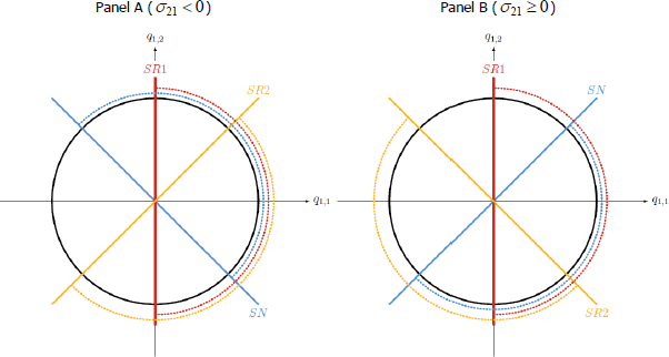
Notes: This figure depicts the identified set for q1 = (q1,1, q1,2) under the identifying restrictions described in the text and assuming that and (Panel A) or 0.5 (Panel B). The black circle is the unit circle. The coloured lines represent the boundaries of the half-spaces generated by the identifying restrictions: ‘SN’ corresponds to the sign normalisation ‘SR1’ corresponds to the sign restriction ‘SR2’ corresponds to the sign restriction The dashed arcs represent the sets of values of q1 satisfying each individual restriction; the arc of the unit circle where the three dashed arcs overlap is the identified set for q1.
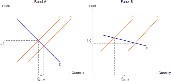
Notes: This figure depicts the shift in the supply curve (from S to S') required to induce a 1 per cent increase in price under differently sloped demand curves (D). The corresponding decrease in quantity is the impulse response to a unit supply shock. This becomes arbitrarily large as the demand curve approaches the horizontal.
Note that unboundedness of the identified set also arises when imposing sign restrictions on multiple columns of Q (i.e. on impulse responses to multiple shocks). When additionally imposing that the impulse responses of both variables to the second shock are positive, the identified set for continues to include zero when and the identified set for is unbounded (see Appendix A.2 for details). Unboundedness of the identified set also occurs when imposing sign restrictions with strict, rather than weak, inequality. Strict inequality restrictions yield identified sets that are open, rather than closed, intervals, but the identified set for remains unbounded when Finally, unboundedness of the identified set does not arise purely due to working in the orthogonal reduced-form parameterisation and defining the unit impulse response as the ratio of impulse responses to standard deviation shocks; that is, it also arises when using a parameterisation that imposes the unit-effect normalisation directly (see Appendix A.3).
This stylised example highlights that the identified set for unit impulse responses may be unbounded if the identified set for the impact response of the normalising variable to a standard deviation shock includes zero. Whether this is the case depends on the values of the reduced-form parameters. The following sections discuss some implications of unboundedness for conducting inference about unit impulse responses.[11]
3.2 Robust Bayesian inference under unboundedness
This section discusses how unboundedness of the identified set affects different inferential outputs (e.g. sets of posterior means or quantiles) under the robust Bayesian approach to inference. To aid explanation, I continue to frame the discussion through the lens of the bivariate model. I also make the simplifying assumption that is supported only on two values of the reduced-form parameters: and where However, the results extend straightforwardly to more general settings. I denote the lower bound of the identified set for when and the posterior probability that The identified set for with posterior probability and it is with posterior probability
Set of posterior means. The set of posterior means, which has bounds equal to the posterior means of the bounds of the identified set, will be unless Consequently, if places positive posterior probability on the event the set of posterior means is completely uninformative about (other than its sign, which is imposed by the sign restrictions).
Sets of posterior quantiles. The set of posterior medians is an interval with lower (upper) bound equal to the posterior median of the lower (upper) bound of the identified set. The median of the upper bound of the identified set is zero regardless of the value of . When the posterior median of the lower bound of the identified set is The set of posterior medians will therefore be bounded. In contrast, when the posterior median of the lower bound of the identified set is so the set of posterior medians is unbounded. By similar logic, the set of posterior -quantiles will be bounded so long as The class of posteriors may therefore still contain useful information about particular posterior quantiles even when the identified set is unbounded with positive posterior probability.
Robust credible intervals. A robust credible interval with credibility can be constructed by taking the quantile of and the quantile of . Whether the robust credible interval is bounded will therefore depend on the credibility level and In particular, boundedness of the robust credible interval requires that the sets of and quantiles are both bounded, which will be the case in the current example if
Posterior lower and upper probabilities. Consider the hypothesis that for some . The posterior lower probability of this hypothesis is equal to the posterior probability that the identified set is contained within the interval . This probability is zero for all x < 0. The posterior upper probability of the hypothesis is equal to the posterior probability that the identified set intersects the interval . The posterior upper probability is one for and is for The set of posterior probabilities for the hypothesis is therefore [0,1] for and is for As approaches zero, so that the identified set is almost always unbounded, the set of posterior probabilities converges to the unit interval for all values of x. In this case, the sign restrictions are not informative about the hypothesis regardless of the value of x. In contrast, as approaches one, the set of posterior probabilities converges to zero for sufficiently negative values of x (i.e. for ). In this case, ‘large’ responses are assigned low posterior probability regardless of the choice of conditional prior.
Summary. This discussion illustrates that it is possible to extract useful information about the impulse responses to a unit shock using the robust Bayesian approach to inference when the identified set is unbounded with positive posterior probability. Moreover, understanding how often the identified set is unbounded (in terms of posterior probability) is valuable for understanding which inferential outputs themselves will be unbounded, and thus for gauging the informativeness of the identifying restrictions.
3.2.1 Frequentist validity
For general set-identified models, Giacomini and Kitagawa (2021) provide high-level conditions under which their robust Bayesian approach to inference has a valid frequentist interpretation, in the sense that the set of posterior means is consistent for the true identified set (i.e. the identified set when is equal to its true value, ) and the robust credible interval has correct frequentist coverage for the true identified set. In the context of SVARs and when the parameter of interest is an impulse response to a standard deviation shock, Giacomini and Kitagawa provide sufficient conditions under which these high-level conditions will hold. In particular, the set of posterior means can be interpreted as a consistent estimator of the true identified set if the identified set is convex and continuous at Additionally, if the end points of the identified set are differentiable in at and have non-zero derivatives, the robust credible interval has valid frequentist coverage of the true identified set.
When the parameter of interest is a unit impulse response, the high-level conditions for frequentist validity of the robust Bayesian approach are not necessarily satisfied. For example, these conditions include the assumption that the true identified set is bounded. Consequently, the robust Bayesian approach to inference is not guaranteed to have an asymptotically valid frequentist interpretation when the parameter of interest is a unit impulse response.
To illustrate, consider the bivariate model and assume that is such that so the true identified set is unbounded. For values of in a small neighbourhood of and so naively applying the robust Bayesian approach in this case will almost surely yield a robust credible interval of asymptotically. Clearly, this interval always (weakly) includes the true identified set, so the asymptotic frequentist coverage probability will be trivially equal to one (i.e. the robust credible interval is conservative).[12]
3.3 Frequentist estimation under unboundedness
Unboundedness may also arise when estimating or conducting inference about unit impulse responses in a frequentist framework. Let be the MLE of If is such that a frequentist estimate of the identified set for – which simply plugs the MLE of into the expression for the identified set given in Section 3.1 – will be bounded. In contrast, if is such that a frequentist estimate of the identified set for will be unbounded.
4. Checking for Unboundedness in SVARs
Understanding how often the identified set is bounded is crucial for understanding which inferential outputs (e.g. robust credible intervals) are themselves bounded, and thus for gauging the informativeness of the identifying restrictions. This section explains how to check whether identified sets for unit impulse responses may be unbounded in the general setting of an n -dimensional SVAR with dynamics and where there are both sign and zero restrictions on the structural parameters. In this general setting, analytical expressions for identified sets are not usually available and it is necessary to approximate the bounds of the identified set numerically. In practice, I recommend that researchers compute and report the posterior probability that zero is included within the identified set for the normalising impulse response, since this tells us which inferential outputs are guaranteed to be bounded.
In the n -variable SVAR (described in Section 2), assume that the sign restrictions include the restriction that the impact response of the first variable to the first shock is non-negative, For example, in the context of estimating the effects of monetary policy shocks, this restriction would require that a positive monetary policy shock (the first shock) does not decrease the federal funds rate (the first variable) on impact. Such a restriction seems natural in empirical settings. The identified set for will be unbounded only if the identified set for includes zero (or, equivalently, is guaranteed to be bounded if does not contain zero).[13] This will be the case if there exists Q satisfying the zero restrictions, a ‘binding’ version of the sign restriction on and any remaining sign restrictions. The following proposition formalises this claim.
Proposition 4.1. (Necessary condition for unbounded ) Assume interest is in the impulse response to a unit shock in the first variable, at some fixed and finite horizon h. The identified set for is unbounded only if
Proposition 4.1 provides a necessary condition for to be unbounded. Intuitively, if the identified set for does not contain zero, it is not possible to construct a sequence for Q converging to the point where such that diverges. If the identified set for includes zero, it may be possible to construct such a sequence. However, this condition does not guarantee that is unbounded and hence is not sufficient. To give an example, consider extending the bivariate model of Section 3 to allow for dynamics:
Assume that B1 is diagonal with diagonal elements diag(B1) = (b11, b22)′. When the identified set for includes zero. However, the identified set for is , which is finite for any b11 and finite h.[14]
In what follows, I discuss how to check whether includes zero, in which case may be unbounded. First, consider imposing a set of sign and zero restrictions constraining q1 only, and The following proposition states a sufficient condition for the identified set for to include zero in this setting.
Proposition 4.2. (Sufficient condition for to include zero.) Assume that any sign and zero restrictions constrain q1 only, is contained within the set of sign restrictions and the number of zero restrictions in satisfies If then
The sufficient condition in Proposition 4.2 is easily verifiable; it simply requires counting the number of identifying restrictions imposed. When the total number of identifying restrictions is no more than the number of endogenous variables in the VAR, the identifying restrictions cannot rule out the possibility that the first variable does not respond to its own shock on impact. Proposition 4.1 then implies that the identified set for a unit impulse response may potentially always be unbounded, and the identifying restrictions may be extremely uninformative about these impulse responses.
The assumption that rules out point identification of q1 (and thus any impulse response to the first shock).[15] If the set of sign restrictions were to exclude the restriction a sufficient condition for would be because one could augment the sign restrictions with and then apply Proposition 4.2. Although Proposition 4.2 only applies when the identifying restrictions constrain a single column of Q, this is the case in many empirical applications; examples include Uhlig (2005) and Arias et al (2019) (see also the references in Gafarov et al (2018)). While the condition is unlikely to hold in applications that impose dynamic sign restrictions (i.e. sign restrictions at multiple horizons), these restrictions are not always imposed. For example, the condition is satisfied in Arias et al (2019), who identify a monetary policy shock by imposing sign and zero restrictions on elements of A0 (see Section 5). To identify an unconventional monetary policy shock, Gafarov et al (2018) impose four restrictions (one zero restriction and three signs restrictions) in a four-variable system. Beaudry, Nam and Wang (2011) identify an ‘optimism’ shock by imposing two restrictions (one zero restriction and one sign restriction) in a five-variable system.
When whether it is possible to construct q1 satisfying and the remaining identifying restrictions depends on the reduced-form parameters. Geometrically, the condition and the zero restrictions are jointly satisfied when q1 lies in an (n – f – 1)-dimensional hyperplane that is orthogonal to and the rows of , while the remaining sign restrictions require q1 to lie within the intersection of s – 1 half-spaces. The identified set for will include zero if and only if the intersection of this hyperplane and these half-spaces is non-empty. When s + f > n, the hyperplane and half-spaces are not guaranteed to intersect; whether they intersect depends on the values of the reduced-form parameters, which determine the orientations of the hyperplane and half-spaces.
As a simple example of applying Proposition 4.2, consider the bivariate model of Section 3. Here, s = 3 > 2 = n, so the condition in Proposition 4.2 is not satisfied and zero is not necessarily included within the identified set for ; in particular, zero is excluded when Removing the restriction means that s = n = 2, so the condition in Proposition 4.2 is satisfied and the identified set for includes zero regardless of the sign of Geometrically, when s = n, the intersection of the half-spaces generated by the sign restrictions always includes the boundary of the half-space representing the restriction (i.e. the hyperplane ). Graphically, one can see this by deleting the line ‘SR2’ in Figure 1.
When the conditions in Proposition 4.2 do not hold (i.e. when s + f > n or the identifying restrictions constrain multiple columns of Q), it is necessary to check whether includes zero to determine whether may be unbounded. The following proposition formulates a necessary and sufficient condition for to include zero. I subsequently discuss how to check this condition in practice.
Proposition 4.3. (Necessary and sufficient condition for .) Let represent an augmented set of zero restrictions that includes a ‘binding’ version of the sign restriction with and let collect the remaining sign restrictions. The identified set for includes zero if and only if the identified set for Q given the augmented set of restrictions, is non-empty.
The rationale underlying Proposition 4.3 is straightforward, so I omit a formal proof. If is non-empty, there exists a value of Q satisfying the identifying restrictions (i.e. within ) such that If is empty, there cannot be a value of Q within such that . An implication of the proposition is that one can check whether contains zero by applying existing numerical algorithms to check whether is non-empty. For example, in the case where there are sign and zero restrictions constraining q1 only, Algorithm 4.1 in Read (2022) can be applied.[16] In the general case where the identifying restrictions (potentially nonlinearly) constrain multiple columns of Q, one can check whether is non-empty by drawing from a uniform distribution over (e.g. using the algorithms in Arias et al (2018) or Giacomini and Kitagawa (2021)) until a draw is obtained satisfying the remaining sign restrictions. If no such draw can be obtained after a large number of draws, this suggests that is empty, in which case must be bounded.
Given draws of from its posterior distribution and having checked whether contains zero at each draw, one can determine whether different inferential outputs are guaranteed to be bounded. Remark 4.1 relates the posterior probability that includes zero to the boundedness of different summaries of the robust Bayesian class of posteriors for .
Remark 4.1. Let be the posterior probability that excludes zero (in which case the identified set for is guaranteed to be bounded by Proposition 4.1) and assume the parameter of interest is Let Then:
- if the set of posterior means is bounded;
- if the set of posterior -quantiles is bounded; and
- if the robust credible interval with credibility , constructed by taking the quantile of and the quantile of , is bounded.
In practice, I recommend that researchers report since doing so makes it clear which inferential outputs are guaranteed to be bounded, and thus is important for understanding the informativeness of the identifying restrictions. For example, if the 68 per cent robust credible interval is guaranteed to be bounded, whereas the 90 per cent robust credible is not necessarily bounded. In this example, reporting a 68 per cent (robust) credible interval (as is common in the literature using set-identified SVARs) may be misleading about the informativeness of the restrictions; presumably, some researchers would be interested in knowing that there is potentially non-trivial posterior probability assigned to infinitely large responses.
5. The Effects of a 100 Basis Point Federal Funds Rate Shock
This section illustrates the empirical relevance of the issues discussed above by estimating the macroeconomic effects of a 100 basis point shock to the federal funds rate under different sets of identifying restrictions that have been used in the literature.
I use the reduced-form VAR considered in Uhlig (2005), Antolín-Díaz and Rubio-Ramírez (2018) and Arias et al (2019). The model's endogenous variables are real GDP (GDPt), the GDP deflator (GDPDEFt), a commodity price index (COMt), total reserves (TRt), non-borrowed reserves (NBRt) (all in natural logarithms) and the federal funds rate (FFRt). I order the variables such that yt = (FFRt, GDPt, GDPDEFt, COMt, TRt, NBRt)', so is the impact response of the federal funds rate to a monetary policy shock. The data are monthly and run from January 1965 to November 2007.[17] The VAR includes 12 lags of the variables and a constant. I assume a Jeffreys' prior over the reduced-form parameters, so This means that the posterior for is a normal-inverse-Wishart distribution, from which it is straightforward to obtain independent draws (e.g. Del Negro and Schorfheide 2011).
The papers listed above conduct Bayesian inference under a uniform prior for Q and primarily present impulse responses to a standard deviation monetary policy shock.[18] In contrast, I focus on the impulse responses to a 100 basis point monetary policy shock and assess the sensitivity of posterior inferences to the choice of prior by conducting robust Bayesian inference. Appendix C describes the numerical algorithms used to implement the inferential procedures applied in this section.
First, I consider the identifying restrictions proposed in Arias et al (2019), who impose sign and zero restrictions on the structural equation for the federal funds rate, which they interpret as a monetary policy reaction function. The restrictions impose that the coefficients on TRt and NBRt in the structural equation for FFRt are zero, which means that the Federal Reserve does not react to changes in reserves when setting the federal funds rate. They also impose sign restrictions on the coefficients of GDPt and GDPDEFt such that the Federal Reserve does not increase the federal funds rate in response to lower output or prices, which is consistent with the types of policy rules typically specified in New Keynesian dynamic stochastic general equilibrium (DSGE) models. The impact response of FFRt to the monetary policy shock is restricted to be non-negative, so that a monetary policy shock does not decrease FFRt on impact, which seems natural. I denote this set of identifying restrictions as Restriction (1).
Figure 3 presents the impulse responses of FFRt and GDPt to a 100 basis point monetary policy shock obtained under Restriction (1) and a conditionally uniform prior for Q . The 68 per cent (equi-tailed) credible intervals include declines in output of close to 4 per cent and the 90 per cent confidence intervals include declines in output exceeding 10 per cent, so there is considerable posterior probability assigned to very large declines in output.
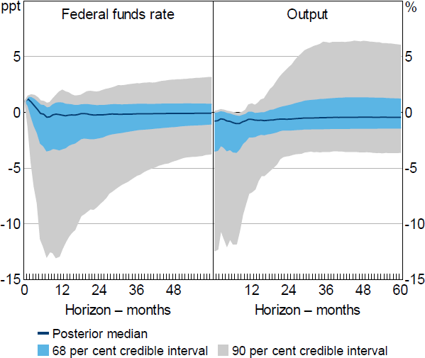
Note: Results obtained under the identifying restrictions in Arias et al (2019); based on 10,000 draws from the posterior of the reduced-form parameters.
The very wide credible intervals suggest that the identifying restrictions are quite uninformative about the output response to a 100 basis point monetary policy shock. However, even these very wide credible intervals severely overstate the informativeness of the restrictions. The restrictions include four sign restrictions (including the sign normalisation on the (1,1) element of A0) and two zero restrictions, so the total number of restrictions is equal to the number of variables in the VAR. This means that the sufficient condition in Proposition 4.2 is satisfied, and zero is always included within the identified set for the impact response of the federal funds rate; in other words, the identifying restrictions cannot rule out the possibility that the federal funds rate does not respond to a standard deviation monetary policy shock on impact. In turn, this suggests that identified sets for unit impulse responses have the potential to be unbounded for all draws of . Examining the approximated bounds of the identified sets for the output responses to a 100 basis point shock suggests that these identified sets are indeed unbounded at every draw, which in turn suggests that the robust credible intervals are unbounded at all credibility levels.[19] The shape of the posterior distribution under the standard approach to inference therefore appears to be driven entirely by the conditional prior.
Next, I combine the restrictions from Arias et al (2019) with the sign restrictions on impulse responses proposed in Uhlig (2005). These sign restrictions impose that the impulse response of FFRt+h to the monetary policy shock is non-negative and the impulse responses of GDPDEFt+h, COMt+h and NBRt+h are non-positive for h = 0,1,..,5.[20] I refer to this set of restrictions as Restriction (2). Under a conditionally uniform prior, the additional sign restrictions appreciably tighten the posterior distribution of the impulse responses to a 100 basis point shock (Figure 4). The posterior median suggests that output falls by a maximum of around 0.4 per cent about two years after the shock and the 68 per cent credible intervals no longer contain extremely large output responses; for example, at the two-year horizon the credible intervals span declines in output of 0.1-0.6 per cent. However, I discuss below that these results are highly sensitive to the choice of conditional prior.
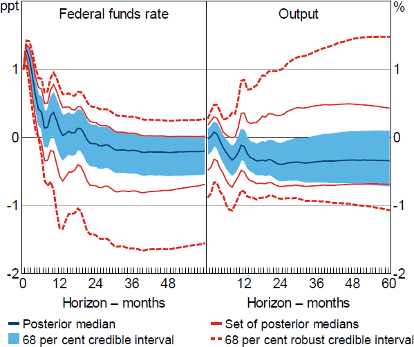
Note: Results obtained under a combination of the identifying restrictions in Uhlig (2005) and Arias et al (2019); based on 10,000 draws from the posterior of the reduced-form parameters.
Under these restrictions, there are 2 zero restrictions and 27 sign restrictions, so the sufficient condition in Proposition 4.2 is not satisfied. This means that the identified set for the impact response of the federal funds rate does not necessarily include zero. I therefore numerically check whether the identified set for includes zero at each draw from the reduced-form posterior. The identified set for includes zero in only 0.06 per cent of draws from the posterior, which implies that the identified sets for the impulse responses to a 100 basis point shock are guaranteed to be bounded with very high posterior probability. It follows that the set of posterior medians is guaranteed to be bounded, as are robust credible intervals at conventional credibility levels (see Remark 4.1). However, the set of posterior medians for the output response includes zero at essentially all horizons, and the 68 per cent robust credible intervals for the output response include both large negative and large positive responses. Hence, the data and identifying restrictions are consistent with either relatively large decreases or increases in output following a 100 basis point shock, and the identifying restrictions are reasonably uninformative about the output response.
These results indicate that much of the apparent information in the standard Bayesian posterior under Restriction (2) is contributed by the conditional prior rather than the data and identifying restrictions, and posterior inferences are sensitive to the choice of conditional prior. To quantify the information contributed by the conditional prior, Giacomini and Kitagawa (2021) suggest reporting the ‘prior informativeness’ statistic; this measures the fraction that the credible interval is tightened (relative to the robust credible interval) by choosing a particular conditional prior. The prior informativeness statistic for the output response is around 70 per cent for the horizons considered (i.e. the 68 per cent credible intervals are around 30 per cent as wide as the 68 per cent robust credible intervals).
Finally, I add the ‘narrative restrictions’ proposed in Antolín-Díaz and Rubio-Ramírez (2018) to Restriction (2). I refer to this set of restrictions as Restriction (3). Narrative restrictions are restrictions on functions of the structural shocks in specific periods (as opposed to restrictions on functions of the structural parameters) that represent information about the nature of the shocks hitting the economy during particular historical episodes.[21] The specific narrative restrictions imposed are that the monetary policy shock was positive and was the ‘overwhelming’ contributor to the forecast error in the federal funds rate in October 1979. This is the month in which the Federal Reserve unexpectedly and dramatically raised the federal funds rate following Paul Volcker becoming chairman, and is widely considered an example of a monetary policy shock (e.g. Romer and Romer 1989).
Under Restriction (3), the identified set for the impact response of the federal funds rate excludes zero in 100 per cent of draws from the reduced-form posterior. Consequently, the set of posterior medians and the robust credible intervals are bounded at all credibility levels. The set of posterior medians for the output response excludes zero at most horizons and the 68 per cent robust credible intervals are substantially narrower than under Restriction (2) (Figure 5). Nevertheless, the robust credible intervals continue to include zero at all horizons and the choice of conditional prior contributes a large share of the information contained in the posterior; the prior informativeness statistic for the output response ranges from around 70 per cent at shorter horizons to around 50 per cent at longer horizons.
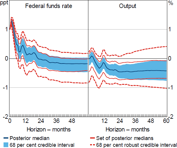
Note: Results obtained under a combination of the identifying restrictions in Uhlig (2005), Antolín-Díaz and Rubio-Ramírez (2018) and Arias et al (2019); based on 1,000 draws from the posterior of the reduced-form parameters.
Table 1 tabulates the posterior lower and upper probabilities that output falls by more than a given threshold x at selected horizons. Under Restriction (2), the posterior lower and upper probabilities that the output response is negative include both small values and values close to one at all horizons, which indicates that the data and identifying restrictions are fairly uninformative about the sign of the output response. In contrast, under Restriction (3), the posterior lower probability that the output response is negative at the two-year horizon is around 75 per cent and the posterior upper probability is 100 per cent. The hypothesis that output declines following a 100 basis point monetary policy shock therefore receives reasonably high posterior probability uniformly over the class of posteriors that are consistent with Restriction (3). Both sets of identifying restrictions effectively rule out relatively large declines in output following a 100 basis point shock; for example, under Restriction (3), the posterior lower probability that output declines by more than 1 per cent two years after the shock is zero and the posterior upper probability is only 6 per cent.
The existing literature contains a wide range of estimates for the output effects of a 100 basis point shock to the federal funds rate; for example, Ramey (2016) reports a range of existing estimates for the trough in the response of output under different samples, specifications and approaches to identification. These estimates range from as low as 0.6 per cent to as high as 5 per cent. The results in Table 1 are broadly consistent with the output effects of monetary policy lying towards the smaller end of the range of existing estimates, in the sense that relatively large output declines are assigned low posterior probability regardless of the choice of conditional prior.
| Horizon | Threshold | ||||||||
|---|---|---|---|---|---|---|---|---|---|
| Lower probability (%) | Upper probability (%) | ||||||||
| 0 | −0.25 | −0.5 | −1 | 0 | −0.25 | −0.5 | −1 | ||
| Restriction (2) | |||||||||
| Impact | 0.00 | 0.00 | 0.00 | 0.00 | 0.95 | 0.75 | 0.48 | 0.10 | |
| One year | 0.13 | 0.01 | 0.00 | 0.00 | 0.99 | 0.84 | 0.48 | 0.06 | |
| Two years | 0.27 | 0.11 | 0.03 | 0.00 | 1.00 | 1.00 | 0.93 | 0.07 | |
| Three years | 0.23 | 0.11 | 0.04 | 0.00 | 1.00 | 0.99 | 0.88 | 0.11 | |
| Four years | 0.23 | 0.12 | 0.05 | 0.00 | 1.00 | 0.98 | 0.80 | 0.15 | |
| Restriction (3) | |||||||||
| Impact | 0.00 | 0.00 | 0.00 | 0.00 | 0.95 | 0.73 | 0.45 | 0.04 | |
| One year | 0.27 | 0.03 | 0.00 | 0.00 | 0.99 | 0.84 | 0.47 | 0.04 | |
| Two years | 0.76 | 0.36 | 0.08 | 0.00 | 1.00 | 1.00 | 0.93 | 0.06 | |
| Three years | 0.64 | 0.33 | 0.11 | 0.01 | 1.00 | 0.99 | 0.88 | 0.10 | |
| Four years | 0.57 | 0.30 | 0.12 | 0.01 | 1.00 | 0.98 | 0.79 | 0.13 | |
| Note: Posterior lower (upper) probability is the smallest (largest) posterior probability obtainable within the class of posteriors consistent with the identifying restrictions. | |||||||||
6. Ruling Out Unboundedness Using Alternative Restrictions
In the context of estimating the effects of monetary policy, the identified set for the impulse responses to a 100 basis point shock may be unbounded when the identified set for the impact response of the federal funds rate to a standard deviation monetary policy shock includes zero. Imposing sign, zero or narrative restrictions of the types considered in Section 5 can indirectly rule this possibility out. This section discusses alternative restrictions that could potentially be used to rule out the possibility that the monetary policy shock has no impact effect on the federal funds rate. Although this discussion is framed in the context of monetary policy, it also applies more generally to other settings.
6.1 Direct bounds on impulse responses
One possibility is to directly restrict the impact response of the federal funds rate to a standard deviation monetary policy shock so that it is greater than some (strictly positive) number (i.e. where is a specified scalar). However, it seems difficult to justify such restrictions on the basis of economic theory – what is the smallest plausible impact effect of a ‘standard deviation’ monetary policy shock on the federal funds rate? Restrictions of this type could potentially be justified on the basis of prior estimates (e.g. from other SVARs or from estimated DSGE models), but these prior estimates may themselves be based on assumptions that lack credibility. Alternatively, one could impose bounds on the responses of variables to a unit shock such that unbounded impulse responses are ruled out by assumption (e.g. ).[22] However, it seems similarly difficult to come up with hard bounds on the responses of variables to a 100 basis point shock without these bounds being somewhat arbitrary. Moreover, in either case, when identified sets are unbounded in the absence of such restrictions, inferences may be highly sensitive to changes in the imposed bounds.
To illustrate, return to the bivariate example of Section 3 and consider additionally imposing that for some . When and , the identified set for is [23]
The additional restriction therefore results in the identified set being bounded; in the absence of this restriction (or in the limit as approaches zero from above), the identified set is However, the lower bound of the identified set is sensitive to the choice of particularly when is small; the derivative of the lower bound tends to as approaches zero from above. Setting to some small positive number to rule out an unbounded identified set for may therefore yield an identified set that is highly sensitive to the choice of .
6.2 Bounds on the forecast error variance decomposition
Rather than directly restricting the impact effect of the monetary policy shock on the federal funds rate, one could instead consider restricting the one-step-ahead forecast error variance decomposition (FEVD) of the federal funds rate with respect to the monetary policy shock. This is the contribution of the monetary policy shock to the one-step-ahead forecast error variance (FEV) of the federal funds rate. Such restrictions may indirectly rule out the possibility that the monetary policy shock has no impact effect on the federal funds rate; intuitively, a strictly positive lower bound on the contribution of the monetary policy shock to the one-step-ahead FEV of the federal funds rate means that the impact effect of the shock itself must be strictly positive.
More formally, the horizon- h FEVD of the i th variable with respect to the j th shock is
The impact effect of the j th shock on the i th variable is zero if and only if so bounding away from zero indirectly bounds the impact response away from zero. However, as in the case where the normalising impulse response is directly bounded away from zero, the identified set obtained under some small lower bound on the FEVD will also be sensitive to the choice of this lower bound when the identified set is unbounded in the absence of this restriction (see Appendix A.5 for an analysis of this case in the context of the bivariate model). Volpicella (2022) proposes imposing bounds on the FEVD, where the bounds are elicited from a range of estimated DSGE models. However, if the assumptions underlying the DSGE models that are used to elicit these bounds lack credibility, the derived bounds on the FEVDs will also lack credibility.
7. Conclusion
In SVARs that are set identified using sign and/or zero restrictions, the identified set for the impulse responses to a unit shock may be unbounded. These restrictions therefore have the potential to be extremely uninformative about the effects of unit shocks. However, it may still be possible to draw useful inferences about impulse responses to a unit shock when the identified set is unbounded with positive posterior probability. Ultimately, I argue that researchers should transparently communicate about the extent to which identified sets are unbounded and what this means about the informativeness of their identifying restrictions.
The empirical exercise in this paper demonstrates the importance of these issues. The identifying restrictions on the systematic component of monetary policy considered in Arias et al (2019) never rule out the possibility that the federal funds rate does not respond on impact to a standard deviation monetary policy shock. As a consequence, the identified set for the output response to a 100 basis point monetary policy shock appears to be unbounded at all horizons and for all values of the reduced-form parameters. The identifying restrictions are therefore extremely uninformative about the magnitude of these impulse responses, standard Bayesian inference is misleading about the information contained in the data given the identifying restrictions, and posterior inferences are sensitive to the choice of conditional prior for the orthonormal matrix.
After additionally imposing the sign restrictions on impulse responses from Uhlig (2005), the identified set is bounded with very high posterior probability; nevertheless, the identifying restrictions are quite uninformative about the output effects of a 100 basis point monetary policy shock and posterior inferences remain sensitive to the choice of prior. Adding the narrative restrictions from Antolín-Díaz and Rubio-Ramírez (2018) yields a bounded identified set in 100 per cent of draws from the reduced-form posterior and leads to more informative inference about the output effects of the shock; however, it remains the case that a large share of the information in the posterior is contributed by the unrevisable component of the prior. The latter two sets of restrictions effectively rule out large declines in output following a 100 basis point shock. It is therefore possible to draw useful inferences about the effects of US monetary policy under set- identifying restrictions even though these restrictions may sometimes be extremely uninformative.
Appendix A: Derivations for Bivariate SVAR
A.1 Sign restrictions on impulse responses
This appendix derives the identified sets for the impulse responses to a unit shock under the sign restrictions on impulse responses presented in Section 3.
In the absence of any identifying restrictions, the identified set for (the matrix of impact impulse responses) is
and the identified set for A0 is
The impact response of the second variable to a shock that raises the first variable by one unit is
Consider the sign restrictions that the impulse response of the first variable to the first shock is non-negative and the impact response of the second variable to the first shock is non-positive , plus the sign normalisation Under this set of restrictions, is restricted to lie within the following set:
There are two cases to consider depending on the sign of . If the second set is empty. The first set is equivalent to
This set of inequalities implies that the identified set for is
which lies within the interval The impact response of the first variable to the first shock is The lower bound of the identified set for is negative and the upper bound is positive, so zero lies within this identified set and attains its maximum of one. The upper bound of the identified set for is therefore . The lower bound is attained at one of the end points of the identified set for and therefore satisfies
where: the second line uses the fact that arctan is an odd function and cos is an even function; and the third line uses the fact that cos is increasing over Since arctan is an increasing function, it follows that:
This identified set excludes zero. Since is strictly increasing in over the interval its lower and upper bounds are attained at the end points of the identified set for . Plugging the end points of the identified set for into the expression for yields the identified set for :
which is bounded.
Similarly, if is restricted to lie in the set
The second inequality implies that so the last inequality never binds. The identified set for is therefore
The upper bound of the identified set for is negative. is therefore strictly increasing over the identified set for , and the bounds of the identified set for are attained at the end points of the identified set for :
If is restricted to the set
The first set implies and the second implies so The expression for the identified set for when therefore also applies when . as approaches from above. is strictly increasing over the identified set for , so the upper bound for the identified set for is obtained by evaluating at the upper bound of the identified set for . Consequently,
A.2 Sign restrictions on impulse responses to multiple shocks
If we additionally impose the sign restrictions that and the parameter is restricted to lie within the following set:
Using working similar to that in Appendix A.1, the identified sets for and are given by:
As in the case where there are sign restrictions on the impulse responses to the first shock only, the identified set for includes zero when and the identified set for is unbounded.[24] In the case where , the additional sign restrictions tighten the identified set. In particular, the upper bound is now strictly less than zero (and is a differentiable function of , as discussed in Section 3.2.1).
A.3 Alternative parameterisation
Consider an alternative parameterisation of the bivariate model that directly imposes the unit-effect normalisation: where ,
Let and The structural parameters and reduced-form parameters are related via . Eliminating and from the system of equations yields a single equation in (H12, H21):
Solving for H21 as a function of H12 (using the quadratic formula) yields:
Figure A1 plots the two solutions. Under the sign restrictions and the identified set for (H12, H21) lies in the lower-right quadrant. When (Panel A), the identified set for H21 is bounded. When (Panel B), the identified set for H21 is unbounded, so unbounded identified sets may also arise when the unit-effect normalisation is directly imposed.
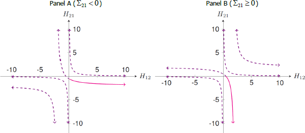
Notes: This figure depicts the solutions to Equation (A19) assuming that and The part of the solution set depicted in the lower-right quadrant of each panel represents the identified set for (H12, H21) under the sign restrictions
A.4 Magnitude restrictions
In addition to the sign restrictions considered in Section 3 and Appendix A.1, consider the restriction that for some Under this set of restrictions, is restricted to lie within the set:
The second set is always empty, since and cannot hold simultaneously when The identified set for is empty if since for all .
If , the first set is equivalent to
The last inequality never binds and the identified set for is
which is contained within the interval is strictly increasing over this interval, so the bounds of the identified set for are attained at the end points of the identified set for . The identified set for is therefore
The lower bound of this identified set, can be expressed as[25]
which converges to as approaches zero from above. The derivative of with respect to is
In the limit as approaches zero from above, this derivative approaches , which implies that the lower bound is extremely sensitive to small changes in when is close to zero.
A.5 Bounds on the FEVD
The FEV of y1t is and the contribution of to the FEV of y1t is The FEVD of y1t with respect to is therefore . Consider imposing the restriction that for some in addition to the sign restrictions considered in Section 3 and Appendix A.1. Under this set of restrictions, is restricted to lie within the following set:
When the first set is equivalent to
The inequalities and never bind and the identified set for is
which is contained within the interval is strictly increasing over this interval, so the bounds of the identified set for are attained at the end points of the identified set for . The identified set for is therefore
The lower bound of this identified set, , can be expressed as
The lower bound converges to as approaches zero from above. The derivative of with respect to is
In the limit as approaches zero from above, this derivative approaches , which implies that the lower bound is extremely sensitive to small changes in when is close to zero.
To summarise, under the additional restriction on the FEVD, the identified set is bounded; in the absence of this restriction (or as converges to zero from above), the identified set is
However, as in the case where the normalising impulse response is directly bounded away from zero, the lower bound of the identified set is sensitive to the choice of , particularly for small values of ; the derivative of the lower bound tends to as approaches zero from above. Setting to some small positive number to rule out an unbounded identified set for will therefore yield an identified set that is highly sensitive to the choice of
Appendix B: Proofs of Propositions
Proof of Proposition 4.1. Assume so there exists such that for all Given that the impulse response horizon h is fixed and finite, for all .[26] There thus exists such that for all It follows that for all , so is bounded.
Proof of Proposition 4.2. Assume that the sign restrictions are ordered such that the first row of corresponds to the sign restriction Let collect the coefficient vectors of the sign and zero restrictions.
First, consider the case where and let represent an orthonormal basis for the null space of . By the rank-nullity theorem, has dimension Thus, it is always possible to construct satisfying by taking any column of . Such a vector clearly satisfies the identifying restrictions with , so .
Now, consider the case where Let represent the coefficients of the zero restrictions augmented with a ‘binding’ version of the sign restriction on , and let represent the coefficients of the remaining sign restrictions (i.e. the last s – 1 rows of ). Since Proposition 4.1 in Read (2022) states that the system of zero and sign restrictions, and , can be transformed into a set of sign restrictions in . Let represent the transformed sign restrictions, where and is obtained from using the transformation described in Read. Corollary 4.1 of Read states that the set will be non-empty if and only if the set is non-empty, in which case I proceed by showing that the set is always non-empty.
If then has dimension so it is always possible to construct satisfying by taking any column of , and the set is non-empty. If there cannot exist such that (since has full rank), so by Gordan's Theorem (e.g. Mangasarian 1994; Border 2020) there must exist such that , so the set is non-empty.
Appendix C: Description of Numerical Algorithms
This section describes the numerical algorithms that I use in the empirical application of Section 5. I first describe at a high level a general algorithm used to conduct robust Bayesian inference. I subsequently provide details about how the algorithm is implemented under the different sets of identifying restrictions.
Algorithm C1 (robust Bayesian inference). Assume the parameter of interest is . For k = 1,...,K:
Step 1: Draw from
Step 2: Check whether is empty. If so, return to Step 1. If not, proceed to Step 3.
Step 3: Record whether
Step 4: Compute and
Given the output of Algorithm C1, the set of posterior medians can be approximated by an interval with lower bound (upper bound) equal to the posterior median of A robust credible interval with credibility can be approximated by an interval with lower bound equal to the quantile of and upper bound equal to the quantile of .[27] If D is some hypothesis about (i.e. that it lies within a specified interval), the posterior lower probability assigned to the hypothesis can be approximated by the posterior probability that the identified set is contained entirely within the interval D (i.e. , where 1(.) is the indicator function). The posterior upper probability can be approximated by the posterior probability that the identified set intersects the interval D (i.e. ). To give an example, if the hypothesis of interest is that the output response is weakly negative at horizon h, D = .
How Steps 2, 3 and 4 of Algorithm C1 are implemented depends on whether the identifying restrictions constrain a single column or multiple columns of Q . When the restrictions constrain a single column of Q only (i.e. under Restrictions (1) and (2)), I check whether the identified set is non-empty at each draw of using Algorithm 4.1 in Read (2022).[28] I also check whether is non-empty (and thus whether includes zero) using this algorithm. I approximate the bounds of the identified set at each draw of by obtaining 10,000 draws of Q from a uniform distribution over , computing at each draw of Q and taking the minimum and maximum over the draws of Q .[29] I draw from the uniform distribution over using the Gibbs sampler described in Read (2022).
Restriction (3) includes restrictions on the historical decomposition. The contribution of the j th structural shock to the one-step-ahead forecast error in variable i in period t is The restriction that the monetary policy shock was the ‘overwhelming’ contributor to the observed unexpected change in the federal funds rate means that the absolute contribution of the monetary policy shock to the forecast error in the federal funds rate is greater than the sum of the absolute contributions of all other shocks, or This is a restriction on the historical decomposition that simultaneously constrains all columns of Q. Consequently, it is necessary to numerically approximate whether and are empty using simulation-based algorithms. I approximate identified sets as being empty if I cannot obtain a draw of Q satisfying the (augmented) identifying restrictions after 100,000 draws. When approximating the bounds of the identified set for , draws of Q from the uniform distribution over are obtained using the accept-reject algorithm described in Giacomini et al (2021a). The numerical methods used to obtain the results under these restrictions are computationally burdensome, so I base the results on 1,000 (rather than 10,000) draws of such that the identified set is non-empty.
In generating the results under the conditionally uniform prior, I obtain a single draw of Q from the uniform distribution over at each draw of using the algorithms described above and transform the draws of into impulse responses via .
Appendix D: Additional Empirical Results
Figure D1 presents additional results obtained under Restriction (2) when the horizon over which the sign restrictions are imposed (H) is varied. For H = 2, the identified set for includes zero in only 1.2 per cent of draws from the posterior. However, the set of posterior medians and 68 per cent robust credible intervals for the output response are extremely wide. Increasing H reduces the proportion of draws where the identified set for includes zero: for H = 5 (the assumption in the main text), the identified set includes zero in 0.6 per cent of draws; and for there are no draws where the identified set includes zero. Increasing the number of sign restrictions also appreciably tightens the set of posterior medians and robust credible intervals.
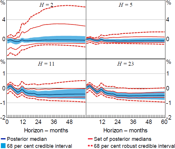
Note: Results obtained under a combination of the identifying restrictions in Uhlig (2005) and Arias et al (2019); H is the horizon over which the impulse responses are restricted; results based on 10,000 draws from the posterior of the reduced-form parameters.
References
Amir-Ahmadi P and T Drautzburg (2021), ‘Identification and Inference with Ranking Restrictions’, Quantitative Economics, 12(1), pp 1–39.
Antolín-Díaz J and JF Rubio-Ramírez (2018), ‘Narrative Sign Restrictions for SVARs’, The American Economic Review, 108(10), pp 2802–2829.
Arias JE, D Caldara and JF Rubio-Ramírez (2019), ‘The Systematic Component of Monetary Policy in SVARs: An Agnostic Identification Procedure’, Journal of Monetary Economics, 101, pp 1–13.
Arias JE, JF Rubio-Ramírez and DF Waggoner (2018), ‘Inference Based on Structural Vector Autoregressions Identified with Sign and Zero Restrictions: Theory and Applications, Econometrica, 86(2), pp 685–720.
Arias JE, JF Rubio-Ramírez and DF Waggoner (2022), ‘Uniform Priors for Impulse Responses’, Federal Reserve Bank of Philadelphia Working Paper WP 22-30.
Bacchiocchi E and T Kitagawa (2021), ‘A Note on Global Identification in Structural Vector Autoregressions’, Centre for Microdata Methods and Practice, cemmap Working Paper CWP03/21.
Baumeister C and JD Hamilton (2015), ‘Sign Restrictions, Structural Vector Autoregressions, and Useful Prior Information’, Econometrica, 83(5), pp 1963–1999.
Baumeister C and JD Hamilton (2018), ‘Inference in Structural Vector Autoregressions When the Identifying Assumptions Are Not Fully Believed: Re-Evaluating the Role of Monetary Policy in Economic Fluctuations’, Journal of Monetary Economics, 100, pp 48–65.
Baumeister C and JD Hamilton (2019), ‘Structural Interpretation of Vector Autoregressions with Incomplete Identification: Revisiting the Role of Oil Supply and Demand Shocks’, The American Economic Review, 109(5), pp 1873–1910.
Baumeister C and JD Hamilton (2022), ‘Advances in Using Vector Autoregressions to Estimate Structural Magnitudes’, Unpublished manuscript, June. Available at <https://drive.google.com/file/d/1gbR6HllbhqkE2msfuApKNe80SPgJe6FY/view>.
Beaudry P, D Nam and J Wang (2011), ‘Do Mood Swings Drive Business Cycles and Is It Rational?’, NBER Working Paper No 17651.
Border KC (2020), ‘Alternative Linear Inequalities’, Unpublished manuscript, California Institute of Technology, v 2020.10.15::09.50. Available at <https://healy.econ.ohio-state.edu/kcb/Notes/Alternative.pdf>.
Del Negro M and F Schorfheide (2011), ‘Bayesian Macroeconometrics’, in J Geweke , G Koop and H van Dijk (eds), The Oxford Handbook of Bayesian Econometrics, Oxford Handbooks, Oxford University Press, Oxford, pp 293–389.
Fry R and A Pagan (2011), ‘Sign Restrictions in Structural Vector Autoregressions: A Critical Review’, Journal of Economic Literature, 49(4), pp 938–960.
Gafarov B, M Meier and JL Montiel Olea (2018), ‘Delta-Method Inference for a Class of Set-Identified SVARs’, Journal of Econometrics, 203(2), pp 316–237.
Galí J (2008), Monetary Policy, Inflation, and the Business Cycle: An Introduction to the New Keynesian Framework, Princeton University Press, Princeton.
Giacomini R and T Kitagawa (2021), ‘Robust Bayesian Inference for Set-Identified Models’, Econometrica, 89(4), pp 1519–1556.
Giacomini R, T Kitagawa and M Read (2021a), ‘Identification and Inference under Narrative Restrictions’, Unpublished manuscript, University College London, 15 February. Available at <https://doi.org/10.48550/arXiv.2102.06456>.
Giacomini R, T Kitagawa and M Read (2021b), ‘Robust Bayesian Analysis for Econometrics’, Centre for Economic Policy Research Discussion Paper DP16488.
Giacomini R, T Kitagawa and M Read (2022a), ‘Narrative Restrictions and Proxies: Rejoinder’, Journal of Business & Economic Statistics, 40(4), pp 1438–1441.
Giacomini R, T Kitagawa and M Read (2022b), ‘Robust Bayesian Inference in Proxy SVARs’, Journal of Econometrics, 228(1), pp 107–126.
Granziera E, HR Moon and F Schorfheide (2018), ‘Inference for VARs Identified with Sign Restrictions’, Quantitative Economics, 9(3), pp 1087–1121.
Hamilton JD (1994), Time Series Analysis, Princeton University Press, Princeton.
Inoue A and L Kilian (2022), ‘The Role of the Prior in Estimating VAR Models with Sign Restrictions’, Unpublished Manuscript, 4 January. Available at <https://drive.google.com/file/d/1HDXiP_b3DTznVhH4bxi8hbo9n1Cs3O2f/view>.
Kilian L (2022), ‘Comment on Giacomini, Kitagawa, and Read's “Narrative Restrictions and Proxies’”, Journal of Business & Economic Statistics, 40(4), pp 1429–1433.
Kilian L and H Lütkepohl (2017), Structural Vector Autoregressive Analysis, Themes in Modern Econometrics, Cambridge University Press, Cambridge.
Kilian L and DP Murphy (2012), ‘Why Agnostic Sign Restrictions Are Not Enough: Understanding the Dynamics of Oil Market VAR Models’, Journal of the European Economic Association, 10(5), pp 1166–1188.
Mangasarian OL (1994), Nonlinear Programming, Classics in Applied Mathematics, 10, corrected republication, Society for Industrial and Applied Mathematics, Philadelphia.
Plagborg-Møller M and CK Wolf (2021), ‘Local Projections and VARs Estimate the Same Impulse Responses’, Econometrica, 89(2), pp 955–980.
Poirier DJ (1998), ‘Revising Beliefs in Nonidentified Models’, Econometric Theory, 14(4), pp 483–509.
Ramey VA (2016), ‘Macroeconomic Shocks and Their Propagation’, in JB Taylor and H Uhlig (eds), Handbook of Macroeconomics: Volume 2A, Handbooks in Economics, Elsevier, Amsterdam, pp 71–162.
Read M (2022), ‘Algorithms for Inference in SVARs Identified with Sign and Zero Restrictions’, The Econometrics Journal, 25(3), pp 699–718.
Romer CD and DH Romer (1989), ‘Does Monetary Policy Matter? A New Test in the Spirit of Friedman and Schwartz’, in OJ Blanchard and S Fischer (eds), NBER Macroeconomics Annual 1989, 4, The MIT Press, Cambridge, pp 121–184.
Rothenberg TJ (1971), ‘Identification in Parametric Models’, Econometrica, 39(3), pp 577–591.
Rubio-Ramírez JF, DF Waggoner and T Zha (2010), ‘Structural Vector Autoregressions: Theory of Identification and Algorithms for Inference’, The Review of Economic Studies, 77(2), pp 665–696.
Stock JH and MW Watson (2016), ‘Dynamic Factor Models, Factor-Augmented Vector Autoregressions, and Structural Vector Autoregressions in Macroeconomics’, in JB Taylor and H Uhlig (eds), Handbook of Macroeconomics: Volume 2A, Handbooks in Economics, Elsevier, Amsterdam, pp 415–525.
Stock JH and MW Watson (2018), ‘Identification and Estimation of Dynamic Causal Effects in Macroeconomics Using External Instruments’, The Economic Journal, 128(610), pp 917–948.
Uhlig H (2005), ‘What Are the Effects of Monetary Policy on Output? Results from an Agnostic Identification Procedure’, Journal of Monetary Economics, 52(2), pp 381–419.
Volpicella A (2022), ‘SVARs Identification through Bounds on the Forecast Error Variance’, Journal of Business & Economic Statistics, 40(3), pp 1291–1301.
Acknowledgements
I thank Christiane Baumeister, Benjamin Beckers, Anthony Brassil, Thomas Cusbert, Thorsten Drautzburg, Luci Ellis, Renée Fry-McKibbin, James Hamilton, Jarkko Jääskelä, Adrian Pagan, Michele Piffer, John Simon and Benjamin Wong for useful discussions and feedback. I also thank conference participants at the Reserve Bank of Australia's 2022 Quantitative Macroeconomics Workshop, 8th Annual Conference of the International Association for Applied Econometrics, 2022 Australasia Meeting of the Econometric Society and 2022 Australian Conference of Economists, as well as seminar participants at the University of Western Australia and Monash University. The views expressed in this paper are my own and do not necessarily reflect the views of the Reserve Bank of Australia. I am solely responsible for any errors.
Footnotes
If the VAR is stable, the identified set for the impulse response to a standard deviation shock is always bounded. The issue of unboundedness is therefore specific to the case where the impulse response of interest is to a unit shock. [1]
I do not make a judgement about the plausibility of the non-response of the policy rate to a monetary policy shock. Rather, I highlight that typical set-identifying restrictions do not necessarily rule out this possibility, and I explore the implications that this has for learning about the impulse responses to unit shocks. Interestingly, conventional macroeconomic theory also does not rule out this non-response; in the textbook New Keynesian model (e.g. Galí 2008), there exists a value for the persistence of the monetary policy shock such that the nominal interest rate does not respond on impact to the shock. [2]
In their online appendix, Baumeister and Hamilton (2018) provide a list of close to 100 studies that estimate set-identified SVARs. [3]
The transformation is not necessarily innocuous in the point-identified setting when conducting frequentist inference. In particular, if the sampling distribution of the estimator for the normalising impulse response has probability mass near zero, the sampling distribution of the estimator for the unit impulse response may be poorly approximated by the usual asymptotic normal distribution; see Stock and Watson (2016) for a heuristic discussion of this point. [4]
The posterior density is the product of the likelihood and the prior density. Conditional on the reduced-form parameters, the likelihood function is flat with respect to the structural parameters, so the posterior will be proportional to the prior. [5]
For example, when estimating the effects of news shocks, it may be natural to normalise a longer-horizon impulse response (Stock and Watson 2018). [6]
See Stock and Watson (2016) or Kilian and Lütkepohl (2017) for overviews of identification in SVARs. See Giacomini and Kitagawa (2021) for more information about the form of and under different types of restrictions. [7]
Inoue and Kilian (2022) and Kilian (2022) argue that posterior sensitivity to the choice of prior is typically not quantitatively important in SVAR applications. However, the evidence that they cite is based on comparing prior and posterior distributions. As discussed in Poirier (1998) and Giacomini, Kitagawa and Read (2021b, 2022a), this comparison is not informative about posterior sensitivity when models are set identified; instead, the relevant measure of posterior sensitivity is the extent to which the posterior changes when the unrevisable component of the prior changes. While the standard Bayesian approach to inference assumes a uniform prior for Q on the basis that this is ‘uninformative’, Baumeister and Hamilton (2015) show that the implicit prior over individual impulse responses is not necessarily uniform (i.e. it may be informative). Arias, Rubio-Ramírez and Waggoner (2022) show that the uniform prior for Q implies a conditional (joint) prior over the vector of impulse responses that is uniform. Giacomini et al (2022a) argue that a uniform prior does not necessarily reflect the absence of prior information about the parameters, which may be better represented by ‘ambiguity’. [8]
Baumeister and Hamilton (2018) also note that the identified set may be unbounded (see their Footnote 4, p 50). [9]
When imposing only the sign normalisation, the identified set for is always in this case, it is possible to approach the point of singularity from the positive or negative direction regardless of the value of When imposing the sign normalisation and the sign restriction the identified set for is always in this case, the point of singularity can be approached from the positive direction only. [10]
Identified sets can also be unbounded when the parameter of interest is the structural coefficient on a particular variable after normalising the coefficient on another variable to equal unity (i.e. the ratio of elements of A0), which may be interpretable as a structural elasticity (e.g. Baumeister and Hamilton 2022). If the identified set for the normalising coefficient includes zero, the identified set for the ratio of coefficients may be unbounded. [11]
In the current bivariate example and when is such that the true identified set is bounded, but the robust credible interval has an asymptotic frequentist coverage probability equal to (i.e. the robust credible interval is conservative). This arises because the upper bound of the identified set is degenerate and is therefore not differentiable in with non-zero derivative. When there are additional sign restrictions on the impulse responses to the second shock, both the lower and upper bound are differentiable in (see Appendix A.2), and the robust credible interval has correct coverage asymptotically. [12]
I abstract from the possibility of imposing sign restrictions with strict inequality (i.e. ). In that case, identified sets will be open intervals (as noted in Section 3.1). Consequently, the identified set for could be unbounded without the identified set for including zero. When allowing for strict inequalities, the identified set for will be unbounded only if the closure of the identified set for includes zero. [13]
I thank Thorsten Drautzburg for suggesting this example. [14]
When rank the identified set for (which, given the sign normalisation, is a singleton when non-empty) excludes zero if rank This condition would be violated in the (unrealistic) instance where the zero restrictions in include the restriction that Note that the condition implicitly rules out the possibility that n = 1, in which case the impulse responses would be trivially point identified. [15]
If f = n – 2 and rank the unit-length vector satisfying is pinned down up to sign; such a vector can be found by computing an orthonormal basis for the null space of If either or then is non-empty. For Algorithm 4.1 in Read (2022) can be applied. [16]
I use the dataset from Antolín-Díaz and Rubio-Ramírez (2018). The monthly series for GDPt and GDPDEFt are obtained by interpolation; see Arias et al (2019) for details. [17]
Uhlig (2005) and Arias et al (2019) present impulse responses to a standard deviation shock. Antolín-Díaz and Rubio-Ramírez (2018) present impulse responses that are normalised such that the median impact response of the federal funds rate is 25 basis points; this differs to the unit-effect normalisation, where the impact response of the federal funds rate is normalised at every draw from the posterior. [18]
For example, the minimum width of the identified set for the impact response of output across the posterior draws is on the order of 100 percentage points and the maximum width is on the order of 108 percentage points. [19]
Uhlig (2005) also considers restricting the impulse responses at shorter and longer horizons than six months. The choice of horizon here does not affect whether the sufficient condition in Proposition 4.2 applies. However, the proportion of draws where the identified set for includes zero varies across the different sets of restrictions, as does the width of the sets of posterior medians and robust credible intervals. Appendix D presents the output responses obtained when the impulse responses are restricted up to horizon [20]
The narrative restrictions are functions of the data through the reduced-form VAR innovations that enter the restrictions (i.e. they do not only depend on ). Consequently, the standard definition of an identified set does not apply; Giacomini, Kitagawa and Read (2021a) instead introduce the concept of a ‘conditional’ identified set, which is the identified set that would be obtained after conditioning on the data that directly enter the narrative restrictions. I refer to the identified set interchangeably with the conditional identified set. [21]
These types of restrictions are sometimes referred to as ‘elasticity restrictions’ (as in Kilian and Murphy (2012)). [22]
If , the identified set is empty. See Appendix A.4 for details about this example. [23]
The identified set for is unbounded when and bounded when [24]
This follows from the fact that [25]
Allowing for arbitrarily large impulse response horizons h would require restricting the support of the reduced-form parameter space such that the infinite-order vector moving average representation of the VAR exists; this will be the case if the eigenvalues of the companion matrix lie inside the unit circle (e.g. Hamilton 1994; Kilian and Lütkepohl 2017). By avoiding this assumption I allow for mildly explosive processes. [26]
This construction of the robust credible interval differs to the shortest robust credible interval in Giacomini and Kitagawa (2021); computing the shortest credible interval requires searching over a grid of possible values, which can be computationally difficult when the identified set is sometimes unbounded. The two constructions of the robust credible interval are similar under Restriction (3) (where the identified set is bounded at every posterior draw). [27]
This algorithm extends an algorithm proposed in Amir-Ahmadi and Drautzburg (2021) to additionally allow for zero restrictions, and requires solving a simple linear program. [28]
Under Restriction (2), the set of posterior medians and robust credible intervals are similar, but a little wider, when approximating the bounds of the identified set using a gradient-based numerical optimisation routine. [29]