RDP 2021-07: Macroprudential Limits on Mortgage Products: The Australian Experience 6. Policy Effects of the Interest-only Limit
July 2021
- Download the Paper 2,356KB
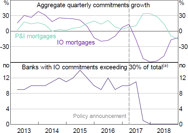
The interest-only mortgage limit, announced at end March 2017, required banks to limit their new IO lending to no more than 30 per cent of total new housing lending. Data are not available for new lending (i.e. mortgage originations), and so we proxy with mortgage commitments. In the aggregate commitments data, the policy effect appears immediate (Figure 7). IO commitments growth falls sharply in 2017:Q2, and in 2017:Q3 and Q4, the number of banks exceeding our proxy of the limit falls to one then zero. This immediate reaction contrasts with the 2-quarter delay in the reaction to the investor policy. Contacts tell us that banks had, by then, developed more capability to control credit growth in targeted products. APRA also provided clearer policy wording. APRA (2019b) writes about the IO policy ‘the experience with the benchmark on lending to investors indicated that the industry would respond most quickly and decisively to a tactical industry-wide regulatory expectation’.

Notes:
The number of banks in the sample varies slightly across periods but is constant from 2016:Q3 to 2018:Q2
(a) May not perfectly align with APRA's assessment of banks meeting the limit
Sources: APRA; Authors' calculations
The results in Sections 6.1 to 6.4 indeed show a faster and neater IO policy reaction than the investor policy reaction. Bank-level growth in IO commitments, and changes in advertised IO rates, react immediately, in 2017:Q2, and large banks substitute into P&I credit one quarter later. Large banks raise advertised IO rates by more than mid-sized banks, and also experience a larger decline in IO commitments growth. Moreover, banks that exceed the IO limit prior to the policy announcement lower their IO commitments growth by significantly more than banks not exceeding the limit. These results are consistent with reports that both banks and APRA benefited from experience with the investor policy while implementing the IO policy.
6.1 Average effects on mortgage commitments
For each sample of banks, the policy significantly reduces targeted credit in the first 3 quarters following the announcement (Table 5). In the full sample, the average bank's IO commitments growth declines 65 percentage points in these 3 quarters (column (a)).[19] Large and mid-sized banks reduce IO commitments growth by around the same overall (columns (d) and (g)), the large banks by a little more. In our commitments proxy, large banks' IO shares tend to exceed the limit by more than mid-sized banks prior to the policy, which explains the larger estimated policy effect for large banks. That is, in the year to 2017:Q1, the average IO share of commitments across large banks lifted from 38 to 41 per cent, while mid-sized banks' same average share lifted from 22 to 24 per cent.
| Sample banks: |
(a) | (b) | (c) | (d) | (e) | (f) | (g) | (h) | (i) | ||
|---|---|---|---|---|---|---|---|---|---|---|---|
| All | Large | Mid-sized | |||||||||
| Mortgage type: | IO | P&I | Total | IO | P&I | Total | IO | P&I | Total | ||
| Policy effects | |||||||||||
| 𝕀(Q2–17) | −0.292*** (0.092) |
−0.099* (0.053) |
−0.166*** (0.042) |
−0.324*** (0.074) |
0.126 (0.099) |
−0.042 (0.052) |
−0.270** (0.110) |
−0.149*** (0.055) |
−0.188*** (0.047) |
||
| 𝕀(Q3–17) | −0.311*** (0.083) |
0.057 (0.041) |
−0.065** (0.025) |
−0.476*** (0.087) |
0.172*** (0.053) |
−0.009 (0.037) |
−0.277*** (0.094) |
0.027 (0.046) |
−0.074*** (0.028) |
||
| 𝕀(Q4–17) | −0.291*** (0.096) |
0.018 (0.053) |
−0.039 (0.051) |
−0.177*** (0.028) |
0.028 (0.036) |
−0.022 (0.023) |
−0.314*** (0.110) |
0.008 (0.062) |
−0.046 (0.061) |
||
| 𝕀(Q1–18) | 0.232 (0.148) |
−0.033 (0.042) |
−0.003 (0.037) |
−0.011 (0.085) |
−0.004 (0.059) |
−0.019 (0.060) |
0.273 (0.171) |
−0.043 (0.050) |
−0.005 (0.043) |
||
| Lagged DVs | 2 | 2 | 2 | 2 | 2 | 2 | 2 | 2 | 2 | ||
| Controls | yes | yes | yes | yes | yes | yes | yes | yes | Yes | ||
| Sample | 788 | 792 | 792 | 168 | 168 | 168 | 620 | 624 | 624 | ||
| Notes: Coefficients from panel regressions, across banks and quarters, of commitments growth on 4 lags of the bank-invariant policy indicator variable. The full equation is in first differences, using Arellano–Bond, with 2 lagged dependent variables to eliminate second order autocorrelation. The control variables are GDP growth, housing price growth, lagged tier 1 capital ratios, lagged deposit funding ratios and a set of seasonal dummy variables. ***, ** and * denote statistical significance at the 1, 5 and 10 per cent levels, respectively. | |||||||||||
In non-targeted credit, large and mid-sized banks' reactions differ, in similar ways to the investor policy reactions. Both curb growth in IO commitments, but only large banks substitute into P&I commitments, so only mid-sized banks reduce total commitments growth. In 2017:Q2 and Q3, large banks experience pick-ups in P&I commitments growth of 13 and 17 basis points, the latter significant, while mid-sized banks experience a significant 15 percentage point decline. The combined effect is that large banks experience no significant change in total commitments growth, while mid-sized banks' total growth declines significantly by around 25 percentage points.
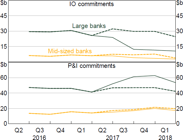
Figure 8 repeats the counterfactuals exercise in Section 5.1 for the IO policy. Large banks' pick-up in commitments for non-targeted (P&I) mortgages is, again, a similar value to their decline in commitments for targeted (IO) mortgages (a bit under $15 billion). Mid-sized banks' non-targeted commitments rise gradually in 2017, but move close to what the estimates suggest would have occurred without the policy.

Sources: APRA; Authors' calculations
6.2 Average effects on advertised interest rates
Large and mid-sized banks both lift IO rates in the first quarter after the policy announcement (Table 6), alongside the declines in IO commitments growth (Section 6.1). Large banks' IO rate rises are larger, in line with their higher IO lending shares prior to the policy (discussed above). At the time, each of the large banks publicly attributed these IO rate rises to the policy (ACCC 2018a). Large and mid-sized banks both reduce IO rates 2 quarters later, when all banks are within our proxy of the limit (Figure 7). The final cumulative effect is still a sizeable IO rate increase – by 34 basis points for the large banks and 16 basis points for the mid-sized banks – which may in part reflect a policy-induced reassessment by banks of the risks of these loans.
The relationships between advertised rate changes and commitments growth, when comparing large and mid-sized banks' reactions, are more intuitive for the IO policy than for the investor policy. Compared to mid-sized banks, large banks initially lift rates by more (in 2017:Q2 and Q3), then lower them by more (in 2017:Q4), and IO commitments growth rates move in the inverse (Table 6, columns (a) and (d); Table 5, columns (d) and (g)). Large banks' non-targeted mortgage commitments, however, appear less sensitive to rates than those of mid-sized banks. In 2017:Q2, both types of banks raise P&I rates, but only mid-sized banks' P&I commitments growth falls.[20] However, this could potentially be explained by large banks' heavier use of rate discounting, which would cause overstated estimates of the true changes in mortgage rates.
| Sample banks: |
(a) | (b) | (c) | (d) | (e) | (f) | |
|---|---|---|---|---|---|---|---|
| Large | Mid-sized | ||||||
| Dependent variable: | IO | P&I | Difference | IO | P&I | Difference | |
| 𝕀(Q2–17) | 0.325*** (0.028) |
0.103*** (0.020) |
0.222*** (0.016) |
0.115*** (0.036) |
0.095*** (0.020) |
0.020 (0.028) |
|
| 𝕀(Q3–17) | 0.106*** (0.031) |
−0.048** (0.022) |
0.154*** (0.015) |
0.097** (0.044) |
0.010 (0.043) |
0.087*** (0.017) |
|
| 𝕀(Q4–17) | −0.090*** (0.029) |
−0.084*** (0.026) |
−0.006 (0.011) |
−0.044** (0.018) |
−0.050** (0.018) |
0.007* (0.004) |
|
| 𝕀(Q1–18) | −0.019 (0.028) |
−0.027 (0.024) |
0.008 (0.014) |
0.043 (0.031) |
−0.010 (0.021) |
0.054*** (0.017) |
|
| Fixed effects | Bank | Bank | Bank | Bank | Bank | Bank | |
| Other controls | yes | yes | yes | yes | yes | yes | |
| R squared | 0.327 | 0.212 | 0.277 | 0.087 | 0.111 | 0.052 | |
| Sample | 164 | 164 | 164 | 501 | 500 | 496 | |
| Notes: Coefficients from panel regressions, across banks and quarters, of change in advertised mortgage rates on 4 lags of the bank-invariant policy indicator variable. All mortgage rates are on investor mortgages. The control variables are GDP growth, housing price growth, lagged tier 1 capital ratios, lagged deposit funding ratios and a set of seasonal dummy variables. Bank fixed effects are included. Standard errors are clustered at the quarter level for the large bank regressions, and at the bank and quarter levels for the mid-sized bank regressions. ***, ** and * denote statistical significance at the 1, 5 and 10 per cent levels, respectively. | |||||||
6.3 Heterogeneous IO-policy effects
In contrast to the investor policy, banks' reactions to the IO policy are clearly related to whether they exceed the limit. In 2017:Q3, banks above the limit reduce IO commitments growth by 27 percentage points more than banks below the limit (Table 7, column (b)).[21] In the same quarter, the linear treatment measure shows that, for every 10 percentage points further above the limit, a bank reduces its IO commitments growth by 14 percentage points more (column (a)).[22] As opposed to the lack of differentiation between banks below and above the threshold seen in Section 6.1, for the IO benchmark banks above react differently to banks below. In addition, banks above the limit have a significantly larger pickup in P&I commitments growth than banks below (columns (c) and (d)). The strong substitution effect for banks above the limit is not surprising, because raising P&I lending is also a way to meet the proportion-based limit on IO lending.
| Dependent variable: |
(a) | (b) | (c) | (d) | (e) | (f) | (g) | (h) | ||||
|---|---|---|---|---|---|---|---|---|---|---|---|---|
| Commitments growth | Rate changes | |||||||||||
| Mortgage type: | IO | P&I | IO | P&I | ||||||||
| Treatment function: | Linear | Binary | Linear | Binary | Linear | Binary | Linear | Binary | ||||
| 𝕀(Q2–17) ×Treatment |
−0.549 (0.496) | −0.095 (0.073) | 1.008*** (0.120) | 0.237*** (0.045) | 0.460*** (0.142) | 0.166*** (0.036) | −0.023 (0.097) | −0.051* (0.026) | ||||
| 𝕀(Q3–17) ×Treatment |
−1.440*** (0.444) | −0.272*** (0.075) | 0.564*** (0.098) | 0.216*** (0.033) | −0.182 (0.269) | −0.055 (0.058) | −0.027 (0.098) | 0.017 (0.019) | ||||
| 𝕀(Q4–17) ×Treatment |
−0.738 (0.761) | 0.029 (0.086) | 0.355 (0.237) | 0.084 (0.056) | −0.170 (0.155) | −0.001 (0.032) | −0.024 (0.065) | 0.006 (0.010) | ||||
| 𝕀(Q1–18) ×Treatment |
−3.079*** (0.803) | 0.012 (0.099) | 0.168 (0.198) | 0.318*** (0.029) | −0.162 (0.143) | 0.000 (0.000) | −0.023 (0.039) | −0.002 (0.004) | ||||
| Fixed effects | Bank & quarter | Bank & quarter | Bank & quarter | Bank & quarter | Bank & quarter | Bank & quarter | Bank & quarter | Bank & quarter | ||||
| Bank controls | yes | yes | yes | yes | yes | yes | yes | yes | ||||
| R squared | 0.368 | 0.359 | 0.346 | 0.346 | 0.210 | 0.211 | 0.727 | 0.728 | ||||
| Sample | 871 | 871 | 874 | 874 | 214 | 214 | 654 | 654 | ||||
| Notes: Coefficients from regressing commitments growth, or change in advertised rates, on 4 lags of the bank-invariant policy indicator variable, each interacted with a ‘treatment’ measure of the bank's distance from the policy limit 2 quarters earlier. The 2 alternative treatment measures are ‘Linear’, equal to the bank's year-ended investor mortgage growth rate (as a decimal) minus 0.1, and ‘Binary’, an indicator for if the bank was exceeding the limit. The regressions include bank and quarter fixed effects. Bank-level controls (capital and deposits) are also included. Standard errors are clustered at the bank and quarter levels. ***, ** and * denote statistical significance at the 1, 5 and 10 per cent levels, respectively. | ||||||||||||
The heterogeneous effect on rates is also clear. In 2017:Q2, every 10 percentage points above the limit translates to a 5 basis point larger IO rate increase (Table 7, column (e)). On average, banks above the limit raise IO rates by 17 basis points more than banks below (column (f)). Also in 2017:Q2, banks above the limit raise P&I rates by 5 basis points less than banks below (column (h)), but there is no significant effect when measuring distance from the limit as a linear rather than binary variable. IO rate effects in subsequent quarters tend to backtrack, but the changes are smaller than the initial policy effects and the coefficients are not significant.
6.4 Placebo regressions
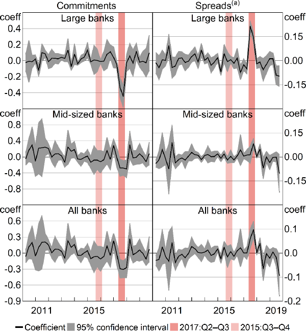
The placebo regression results provide further evidence, in addition to the heterogeneous effect regressions, that the estimated policy effects in Sections 6.1 and 6.2 are true policy effects. In all of the placebo regressions, there are no deviations outside the policy periods that have the size and statistical significance of the estimated policy effects (Figure 9).

Note: (a) Spreads are between IO rates and P&I rates for investor mortgages
Footnotes
The calculation for the cumulative effect on growth is 1 – (1 – 0.292) × (1 – 0.311) × (1 – 0.291). [19]
Large and mid-sized banks also raise rates on P&I mortgages, in 2018:Q1, which is partly undone by subsequent declines. However, this is a by-product of using investor P&I rates, rather than a true policy effect. (We use investor P&I rates to hold the borrower type constant.) Investor P&I commitments growth picked up throughout 2016, while the investor limit was still in place, and these rate rises were likely in response. Repeating the Table 6 regressions but replacing investor P&I rates with occupier P&I rates shows no significant rate rises. [20]
There are also significant policy coefficients in 2018:Q1. However, by this point, all banks except one are below the lagged benchmark (i.e. at 2017:Q3), so the binary treatment measure is unreliable. Further, the linear effect on IO approvals is driven by banks that are well below the threshold and beginning to raise IO approvals again by more than others. [21]
The coefficient of –1.440 corresponds to a bank that is 100 percentage points above the limit, so for a bank 10 percentage points above, the effect is 0.1 × –1.440 = –0.144. [22]